Chapter 6 Factor Models
6.1 The idea behind factor models
In the previous chapter, we looked at the Markowitz Mean-Variance optimisation and introduced its composition. Therein, we derived the model under the consideration of the mean, variance as well as covariance matrix between the individual, observed assets. In the case of n assets, we thus stated that we require n means, n variances and n(n-1)/2 covariances, resulting in a total of 2n + n(n-1)/2 parameters to describe the model. For instance, if we have 1000 assets, then we would require 501’500 parameters to describe the model inherently. Furthermore, we can show that attempting to estimate the model parameters with a sufficient precision is nearly unfeasible using historical price data over time. This is due to the fact that the precision of any variable within an iid setting depends on the square root of the number of observations. Consequently, if the number of observations is insufficiently large, confidence intervals to determine the accuracy of any expected variable value would be deemed redundant. Given the large number of parameters required to describe the model and the number of observations required to estimate the model parameters with sufficient precision, we understand that the Markowitz model is deemed to be a very data intensive model. As a consequence, we need to find simpler models which are less data intensive but can still capture a sufficient amount of the underlying, true asset variation.
Based on this notion, the term Factor Models was primed. These models assume that the correlation between any two assets is explained by systematic factors. That is, the underlying return structure of multiple assets depends on common components which can be represented by quantifiable proxies. Using this assumption, one can restrict attention to only K (non-diversifiable) factors.
Factor models have the advantage that they drastically reduce the number of input variables. Further, they allow to estimate systematic risk components by analysing expected return structures. However, they are purely statistical models and rely on past data. Further, they all assume stationarity.
The aim of factor models is to understand the drivers of asset prices. Broadly speaking, the main concept behind factor investing is that the financial performance of firms depends on distinct factors, whether they are latent or macroeconomic, or related to intrinsic, firm-specific characteristics. Cochrane (2011) states that the first essential question is which characteristics really provide independent information about average returns. Understanding whether the exposure of assets towards common variable(s) can be used to help explain the cross-sectional variation in returns is therein the main emphasis of factor investing.
As we have covered in the lecture, factor models are natural extensions of the Arbitrage Pricing Theory model (APT) introduced by Ross (1976), who assumes that security returns return can be modeled as a linear combination of underlying factors \(f_k\) and that investors operate in functioning security markets which do not allow for the persistence of arbitrage opportunities:
\[ r_{i,t} = \alpha_i + \sum_{i=1}^K \beta_{i,k}f_{t,k} + \epsilon_{i,t} \]
Here, the usual IID setting econometric assumptions hold, implying that \(cov(\epsilon_{i,t},\epsilon_{j,t}) = 0\) and \(cov(\epsilon_{i},f_{i}) = 0\).
A quasi factor-based model is The CAPM. The CAPM is a commonly used model to assess asset returns. Previously, we introduced both the theoretical intuition as well as the practical implementation of the model. We derived how the exposure towards market movements influence stock returns and showed how to compute the underlying framework. Further, we derived options to test the model’s validity and showed that the CAPM does not hold empirically. Consequently, we were able to present that the theoretical foundations of the CAPM are not sufficient to effectively explain the variation in asset returns. This implies that other factors are needed to help explain the remaining variation in asset returns unexplained by the market. To put it in other words, the existence of factors that can explain asset returns further contradicts the validity of the CAPM, which assumes that the variation solely depends on the market portfolio. Consequently, factors are also regarded as anomalies. A quasi factor-based model is The CAPM. The CAPM is a commonly used model to assess asset returns. Previously, we introduced both the theoretical intuition as well as the practical implementation of the model. We derived how the exposure towards market movements influence stock returns and showed how to compute the underlying framework. Further, we derived options to test the model’s validity and showed that the CAPM does not hold empirically. Consequently, we were able to present that the theoretical foundations of the CAPM are not sufficient to effectively explain the variation in asset returns. This implies that other factors are needed to help explain the remaining variation in asset returns unexplained by the market. To put it in other words, the existence of factors that can explain asset returns further contradicts the validity of the CAPM, which assumes that the variation solely depends on the market portfolio. Consequently, factors are also regarded as anomalies.
Importantly, each factor portfolio is a tracking portfolio. That is, the returns on such a portfolio are tracked by the evolution of one particular source of risk but are uncorrelated with other sources of risk.
6.2 The quest of detecting anomalies
How can we thus find such anomalies? As we already mentioned, there is no clear theoretical foundation to the use of certain factors. Mostly, researchers or industry experts consider market movements and attempt to pin down these movements based on correlating characteristics (either micro- or macro-oriented) of the firms under consideration. Usually then, based on these observations, theoretical arguments which suit the given movements are constructed around the anomalies. For instance, Chen Roll and Ross introduced one of the most fundamental multifactor models in 1986 by incorporating macroeconomic variables such as Growth in industrial productiion, inflation expected changes or corporate rated bonds and found a significant effect in the cross-section of returns. Based on their research, Fama and French (1993) created their famous Size and Value portfolio strategies on the observations that small size (measured by market capitalisation) as well as value (measured by high book-to-market ratios) securities outperform their opposite counterparts. Further notable examples include the Momentum strategy (by Jegadeesh and Titman (1993) and Carhart (1997)), Profitability (by Fama and French (2015) and Bouchaud et al. (2019)), Investment (by Fama and French (2015) as well as Hou, Xue, and Zhang (2015)) as well as low-risk (by Frazzini and Pedersen (2014)) or Liquidity factor (by Acharya and Pedersen (2005)).While these factors (i.e., long-short portfolios) exhibit time-varying risk premia and are magnified by corporate news and announcements, it is well-documented (and accepted) that they deliver positive returns over long horizons.
In essence, factors that are shown to hold empirically are manifold. For instance, Chen and Zimmermann (2019) attempt to replicate the 300 most commonly cited factors introduced during the last 40 years and publish the final factors on their website called . Although their work greatly facilitates an improved accessibility of factor investment opportunities, they also show the inherent challenges associated with factor investing. These include, among others:
- The limited possibility to replicate the factor exposure
- The dependence of the variational properties on data-specific idiosyncracies
- The likelihood of p-hacking strategies
- The time-wise dependence on factor exposure
- The destruction of potentially valid factor premia may be due to herding
- The fading of anomalies due to the publication and subsequent reduction of arbitrage opportunities (through re-investment of multiple market participants)
Consequently, although the pool of potentially valid factors is quite large, several of these factors suffer from one or multiple of the aforementioned issues, thereby rendering their empirical validity at least partially questionable. As such, although a multitude of potential characteristics are able to explain asset returns both time-series wise and cross-sectionally, the large-scale use of high-dimensional factor models must be addressed critically.
6.3 The Fama-French Three Factor Model
The perhaps most famous factor model is the Fama-French three-factor model (1993). It was based on observations by the researchers which found that small size (measured by market capitalisation) as well as value (measured by high book-to-market ratios) securities outperform their opposite counterparts. The theoretical reasoning for this were mostly pinned down to risk-based anomalies. For instance, it was argued that small companies outperform their larger counterparts because they are exposed towards a higher liquidation, operational as well as credit based risk, implying that they need to compensate for said risk throughout a higher return structure. Furthermore, the value factor was usually explained through perceptions of future performance based on financing activities, which might also constitute as financial distress assessments.
Fama and French do not only highlight the importance of size and value, but they also develop a method to generate factor portfolios.
Their main strategy is the following. They construct a portfolio of large firms and one of small firms. As break point they use the median size of the firms listed on NYSE to classify all stocks traded on NYSE, Amex and Nasdaq. These portfolios are value weighted. They then construct a zero net investment size factor portfolio by going long the small and going short the big stock portfolio. Further, they construct a Book-to-Market (B2M) exposure by sorting the stocks into low (bottom 30%), medium (middle 40%) and high (top 30%) groups based on B2M.
Based on this, they construct six portfolios based on the intersection of size and B/M sorts:
S/L: Small Stocks with Low B2M
S/M: Small Stocks with Medium B2M
S/H: Small Stocks with High B2M
B/L: Big Stocks with Low B2M
B/M: Big Stocks with Medium B2M
B/H: Big Stocks with High B2M
The returns of the zero-net-investment factors SMB (Small minus Big) and HML (High minus Low) are created from these portfolios
\[ \begin{align} R_{SMB} &= 1/3(R_{S/L} + R_{S/M} + R_{S/H}) - 1/3(R_{B/L} + R_{B/M} + R_{B/H}) \\ R_{HML} &= 1/2(R_{S/H} + R_{B/H}) - 1/2(R_{S/L} + R_{B/L}) \end{align} \]
Based on these factors, the factor betas of the stocks are calculated in a First Pass regression:
\[ E(R_i) - r_f = \alpha_i + \beta_i(E(R_M) - r_f) + \gamma_iE[R_{SMB}] + \delta_iE[R_{HML}] \]
The method used of Fama-French to construct the factors is the most widely adopted approach to create factors. Most of the subsequent factors were created using said approach of sorting stocks into either \(2 \times 3\) or \(2 \times 2\) portfolios. For instance, to construct the Momentum Factor by Jegadeesh and Titman (1996) as well as Carhart (1997), you can use the same approach as for the HML factor, but just double-sort it based on size and the previous Up/Down movements.
6.4 Testing for factor validity
As we discovered, factor investing describes an investment strategy in which quantifiable corporate or macroeconomic data is considered. Therein, the variation in security returns is poised to depend collectively on these characteristics. In order to test for the validity of the underlying characteristic in determining asset returns, we thus need to set the asset returns in a relation to the factor under consideration. The industry surrounding this investment style poses several methods to test said validity, both within time-series as well as cross-sectional settings.
Throughout the subsequent chapter, we will go over the most common techniques to test for factor validity. Throughout, we will cover the theoretical underpinnings, the actual testing strategy as well as the intuition behind each approach. Further, we will illustrate each testing strategy by using code-based examples on the Size Factor first introduced by Fama and French (1993).
6.4.1 Portfolio Sorts
This is the simplest and most widely applied form of factor testing. The idea is straight-forward: We sort portfolios based on the risk factor under consideration into percentiles (e.g. deciles, quintiles). Then, we look at the return and variance structure of each portfolio and compare their structure throughout the individual percentiles to observe whether we see significant differences between them.
In essence, on each date t, we perform the following steps:
- Rank firms according to a criterion (e.g. Market Capitalisation)
- Sort the firms into portfolios based on the criterion (e.g 10 portfolios for decile portfolios)
- Calculate the weights (either equally or value-weighted)
- Calculate the portfolio returns at t+1
The resulting outcome is a time series of portfolio returns for each portfolio j, \(r_t^j\). Then, we identify an anomaly in the following way:
- Construct a Long-Short portfolio strategy by buying the highest and selling the lowest portfolio percentile group
- Conduct a t-test of the long-short strategy
In essence, what we want to observe is the following:
- A monotonous (possibly significant) change (either increase or decrease) in average returns throughout the portfolio sorts
- A significant t-value for the long-short strategy
Based on the literature, if we can observe both, then we can strengthen our assumption that the factor materially affects security returns. The reasoning is the following. We hypothesise that asset returns depend on a common factor. As such, the larger the exposure of a security towards said factor is, the stronger the returns should be affected by the factor. Consequently, the return of assets in higher portfolios should behave differently to that in lower portfolios. Further, if we assume that the factor under consideration influences the return structure of all assets, then we would expect that the effect grows continuously when moving from one portfolio to the other, inducing a monotonous effect throughout our assets.
First, let’s calculate quintile portfolios based on the characteristic
# Load the datasets
Prices_Adj <- read.csv("~/Desktop/Master UZH/Data/A4_dataset_01_Ex_Session.txt", header = T, sep = "\t")
Prices_Unadj <- read.csv("~/Desktop/Master UZH/Data/A4_dataset_04_Ex_Session.txt", header = T, sep = "\t")
Shares <- read.csv("~/Desktop/Master UZH/Data/A4_dataset_03_Ex_Session.txt", header = T, sep = "\t")

# Create Time-Series objects
Prices_Adj_ts <- xts(x = Prices_Adj[,-1], order.by = as.Date(dmy(Prices_Adj[,1])))
Prices_Unadj_ts <- xts(x = Prices_Unadj[,-1], order.by = as.Date(dmy(Prices_Unadj[,1])))
Shares_ts <- xts(x = Shares[,-1], order.by = as.Date(dmy(Shares[,1])))

# Calculate the Returns
Returns_Adj_ts <- Return.calculate(Prices_Adj_ts, method = "discrete")

# Create the market cap Time-Series
Market_Cap_ts <- Shares_ts * Prices_Unadj_ts

# Perform the decile portfolio sorts
## Take the quintile values
quintiles <- c(0.2, 0.4, 0.6, 0.8)
## Create variables indicating the respective 20'th, 40'th, 60'th, 80'th quintile for each month
for (i in quintiles){
  assign(paste0("Market_Cap_Cutoff_", i, "_ts"), matrixStats::rowQuantiles(as.matrix(Market_Cap_ts), probs = i, na.rm = T))
}

# Create the portfolio returns for each quintile
for (i in names(Market_Cap_ts)){
  # First create the market capitalisation of each quintile
  Market_Cap_Q1 <- ifelse(Market_Cap_ts[,i] <= Market_Cap_Cutoff_0.2_ts, 1, NA)
  Market_Cap_Q2 <- ifelse((Market_Cap_ts[,i] > Market_Cap_Cutoff_0.2_ts) & (Market_Cap_ts[,i] <= Market_Cap_Cutoff_0.4_ts), 1, NA)
  Market_Cap_Q3 <- ifelse((Market_Cap_ts[,i] > Market_Cap_Cutoff_0.4_ts) & (Market_Cap_ts[,i] <= Market_Cap_Cutoff_0.6_ts), 1, NA)
  Market_Cap_Q4 <- ifelse((Market_Cap_ts[,i] > Market_Cap_Cutoff_0.6_ts) & (Market_Cap_ts[,i] <= Market_Cap_Cutoff_0.8_ts), 1, NA)
  Market_Cap_Q5 <- ifelse(Market_Cap_ts[,i] > Market_Cap_Cutoff_0.8_ts, 1, NA)
  # Then multiply the Market Cap quintile indicators with the secutity returns
  Return_Market_Cap_Q1  <- stats::lag(Market_Cap_Q1, 1) * Returns_Adj_ts['1991-01-01/2019-12-01', i]
  Return_Market_Cap_Q2  <- stats::lag(Market_Cap_Q2, 1) * Returns_Adj_ts['1991-01-01/2019-12-01', i]
  Return_Market_Cap_Q3  <- stats::lag(Market_Cap_Q3, 1) * Returns_Adj_ts['1991-01-01/2019-12-01', i]
  Return_Market_Cap_Q4  <- stats::lag(Market_Cap_Q4, 1) * Returns_Adj_ts['1991-01-01/2019-12-01', i]
  Return_Market_Cap_Q5  <- stats::lag(Market_Cap_Q5, 1) * Returns_Adj_ts['1991-01-01/2019-12-01', i]

  if (i == "NESN"){
    Return_Market_Cap_Q1_final <- Return_Market_Cap_Q1
    Return_Market_Cap_Q2_final <- Return_Market_Cap_Q2
    Return_Market_Cap_Q3_final <- Return_Market_Cap_Q3
    Return_Market_Cap_Q4_final <- Return_Market_Cap_Q4
    Return_Market_Cap_Q5_final <- Return_Market_Cap_Q5
  }
  else {
    Return_Market_Cap_Q1_final <- cbind(Return_Market_Cap_Q1_final, Return_Market_Cap_Q1)
    Return_Market_Cap_Q2_final <- cbind(Return_Market_Cap_Q2_final, Return_Market_Cap_Q2)
    Return_Market_Cap_Q3_final <- cbind(Return_Market_Cap_Q3_final, Return_Market_Cap_Q3)
    Return_Market_Cap_Q4_final <- cbind(Return_Market_Cap_Q4_final, Return_Market_Cap_Q4)
    Return_Market_Cap_Q5_final <- cbind(Return_Market_Cap_Q5_final, Return_Market_Cap_Q5)
  }
}

# Create mean returns of each portfolio
Mean_Return_EW_Q1_final <- rowMeans(Return_Market_Cap_Q1_final, na.rm = T)
Mean_Return_EW_Q2_final <- rowMeans(Return_Market_Cap_Q2_final, na.rm = T)
Mean_Return_EW_Q3_final <- rowMeans(Return_Market_Cap_Q3_final, na.rm = T)
Mean_Return_EW_Q4_final <- rowMeans(Return_Market_Cap_Q4_final, na.rm = T)
Mean_Return_EW_Q5_final <- rowMeans(Return_Market_Cap_Q5_final, na.rm = T)

# Merge the entire datatframe to one
Dates <- as.Date(dmy(Prices_Adj[,1][14:361]))
## For the normal returns
Mean_Return_EW_quintiles <- as.data.frame(cbind(Dates,
                                                Mean_Return_EW_Q1_final,
                                                Mean_Return_EW_Q2_final,
                                                Mean_Return_EW_Q3_final,
                                                Mean_Return_EW_Q4_final,
                                                Mean_Return_EW_Q5_final))

Mean_Return_EW_quintiles_ts <- xts(x = Mean_Return_EW_quintiles[,-1], order.by = Dates)
colnames(Mean_Return_EW_quintiles_ts) <- c("Quintile 1", "Quintile 2", "Quintile 3", "Quintile 4", "Quintile 5")
## For the cumulative returns
Mean_Return_EW_quintiles_cp <- as.data.frame(cbind(Dates,
                                                cumprod(1+Mean_Return_EW_Q1_final),
                                                cumprod(1+Mean_Return_EW_Q2_final),
                                                cumprod(1+Mean_Return_EW_Q3_final),
                                                cumprod(1+Mean_Return_EW_Q4_final),
                                                cumprod(1+Mean_Return_EW_Q5_final)))

Mean_Return_EW_quintiles_cp_ts <- xts(x = Mean_Return_EW_quintiles_cp[,-1], order.by = Dates)
colnames(Mean_Return_EW_quintiles_cp_ts) <- c("Quintile 1", "Quintile 2", "Quintile 3", "Quintile 4", "Quintile 5")

# Finally, we can plot the relationship
plot_ret <- tidy(Mean_Return_EW_quintiles_ts) %>% ggplot(aes(x=index,y=value, color=series)) + geom_line() +
  scale_color_manual(values=c("tomato3", "khaki3", "lightsteelblue3", "dodgerblue4", "violetred4")) +
ylab("Cumulative Returns") + xlab("Time") + ggtitle("Relationship of Normal Returns on Quintile PF based on Market Cap") +
theme(plot.title= element_text(size=14, color="grey26",
hjust=0.5,
lineheight=1.2), panel.background = element_rect(fill="#f7f7f7"),
panel.grid.major.y = element_line(size = 0.5, linetype = "solid", color = "grey"),
panel.grid.minor = element_blank(),
panel.grid.major.x = element_blank(),
plot.background = element_rect(fill="#f7f7f7", color = "#f7f7f7"), axis.title.x = element_text(color="grey26", size=12),
axis.title.y = element_text(color="grey26", size=12),
axis.line = element_line(color = "black"))

# Finally, we can plot the relationship
plot_cumret <- tidy(Mean_Return_EW_quintiles_cp_ts) %>% ggplot(aes(x=index,y=value, color=series)) + geom_line() +
  scale_color_manual(values=c("tomato3", "khaki3", "lightsteelblue3", "dodgerblue4", "violetred4")) +
ylab("Cumulative Returns") + xlab("Time") + ggtitle("Relationship of Cumulative Returns on Quintile PF based on Market Cap") +
theme(plot.title= element_text(size=14, color="grey26",
hjust=0.5,
lineheight=1.2), panel.background = element_rect(fill="#f7f7f7"),
panel.grid.major.y = element_line(size = 0.5, linetype = "solid", color = "grey"),
panel.grid.minor = element_blank(),
panel.grid.major.x = element_blank(),
plot.background = element_rect(fill="#f7f7f7", color = "#f7f7f7"), axis.title.x = element_text(color="grey26", size=12),
axis.title.y = element_text(color="grey26", size=12),
axis.line = element_line(color = "black"))

plot_ret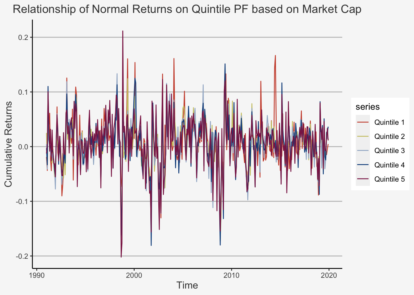
plot_cumret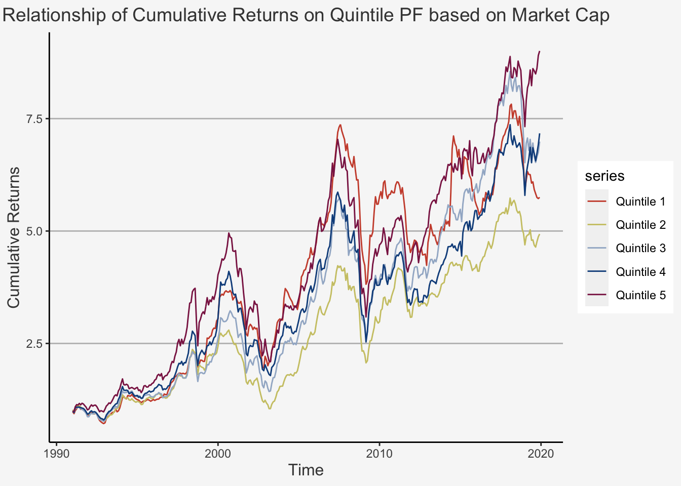
As we can see, there appears to be a strictly increasing trend based on the quintile portfolios. We can confirm this trend by looking at the average returns and their standard deviations.
# Calculate the mean returns
Mean_Return_EW_quintiles_ts <- xts(x = Mean_Return_EW_quintiles[,-1], order.by = Dates)

for (i in names(Mean_Return_EW_quintiles_ts)){
  Mean_Return_EW <- mean(Mean_Return_EW_quintiles_ts['1991-01-01/2019-12-01', i])
  SD_Return_EW <- sd(Mean_Return_EW_quintiles_ts['1991-01-01/2019-12-01', i])
  n_Return_EW <- length(Mean_Return_EW_quintiles_ts['1991-01-01/2019-12-01', i])

  if (i == "Mean_Return_EW_Q1_final"){
    Mean_Return_EW_final <- Mean_Return_EW
    SD_Return_EW_final <- SD_Return_EW
    n_Return_EW_final <- n_Return_EW
  }

  else {
    Mean_Return_EW_final <- cbind(Mean_Return_EW_final, Mean_Return_EW)
    SD_Return_EW_final <- cbind(SD_Return_EW_final, SD_Return_EW)
    n_Return_EW_final <- cbind(n_Return_EW_final, n_Return_EW)
  }
}

# Create the final dataframe
Mean_SD_Size_EW_Quintile_PF <- as.data.frame(rbind(Mean_Return_EW_final, SD_Return_EW_final, n_Return_EW_final))
colnames(Mean_SD_Size_EW_Quintile_PF) <- c("Quintile_1", "Quintile_2", "Quintile_3", "Quintile_4", "Quintile_5")
rownames(Mean_SD_Size_EW_Quintile_PF) <- c("Average Return", "SD Return", "N Observations")

round(Mean_SD_Size_EW_Quintile_PF,4)
## Quintile_1 Quintile_2 Quintile_3 Quintile_4 Quintile_5
## Average Return 0.0060 0.0054 0.0066 0.0067 0.0075
## SD Return 0.0436 0.0406 0.0450 0.0446 0.0482
## N Observations 348.0000 348.0000 348.0000 348.0000 348.0000Finally, we can compute the t-test to check if the average return is statistically different
# Let's create a simple function to calculate the t-test for the average difference
t_test_mean_diff <- function(mean_a, mean_b, sd_a, sd_b, n_a, n_b) {
  t_test <- (mean_a - mean_b) / sqrt(sd_a^2/n_a + sd_b^2/n_b)
  return(t_test)
}

# Try out the formula
t_test_mean_diff(Mean_SD_Size_EW_Quintile_PF$Quintile_5[1],
                 Mean_SD_Size_EW_Quintile_PF$Quintile_1[1],
                 Mean_SD_Size_EW_Quintile_PF$Quintile_5[2],
                 Mean_SD_Size_EW_Quintile_PF$Quintile_1[2],
                 Mean_SD_Size_EW_Quintile_PF$Quintile_5[3],
                 Mean_SD_Size_EW_Quintile_PF$Quintile_1[3])
## [1] 0.444822As we can see, there is no significant difference between the average returns of the high and the low portfolio. This implies, given the IID considerations and the baseline statistical properties assumed, the difference in average returns between the smallest and largest stock portfolio is statistically indistinguishable from zero at conventional levels. Thus, the hypothesis that the average returns are not different from each other cannot be rejected.
6.4.2 Factor Construction
The second approach constitutes the creation of so-called risk-factor mimicking portfolios. These are portfolios which are sorted based on the risk factor of interest but are put relative to each other, depending on the exposure towards the characteristic under consideration. Consequently, we follow a quite similar approach to the portfolio sorts. That is, we:
- First single-sort the assts based on specific characteristics in usually 2 or 3 portfolios
- Double-sort the assets based on the portfolio allocations of the first sort (e.g. Small and Low B2M assets) to obtain the risk-factor mimicking portfolios
- Take the difference between the double-sorted portfolios which are more and which are less exposed towards the given risk factor
The most usual approaches include forming bivariate sorts and aggregating several portfolios together, as in the original contribution of Fama and French (1993). However, some papers also only single-sort the portfolios based on only the respective risk factor. Seldomly, but sometimes appearing, practitioners use n-fold sorting approaches, implying they sort the assets according to n-folds. However, an important caveat with this strategy is the scalability. For instance, let’s look at the n = 3 case, in which we would sort portfolios based on Size, B2M and previous return (used for the Momentum factor). Let’s assume we would sort portfolios based on each characteristics according to above and below median values. In that case, we would create \(2 \times 2 \times 2 = 8\) sorts. For instance, the SMB factor would be:
\[ \begin{equation} SMB = 1/4(R_{SLU} + R_{SHU} + R_{SLD} + R_{SHD}) - 1/4(R_{BLU} + R_{BHU} + R_{BLD} + R_{BHD}) \end{equation} \]
With this strategy, we now interacted the assets based on each characteristic under consideration. For instance, \(R_{SHU}\) is the return of the Small-High-Up portfolio, implying lower than median market capitalisation, higher than median B2M ratio and higher than average past return. It is easy to see that operating on high-dimensional regression settings would quickly render this approach infeasible as the resulting number of created portfolios grows by a factor of \(2^n\) if a complete interaction is to be maintained. And this is if we only keep to sort the portfolios based on median values. Given the large amount of factors that have been proposed throughout the last two decades (currently there are over 300 factors that are argued to explain the return structure of US equities), such an approach would require substantial computational power to enable a high-dimensional factor analysis.
Consequently, let’s follow two approaches in the subsequent factor creation.
- First, we single-sort portfolios based on their market capitalisation and then take their difference to create a Long-Short (LS) Size Portfolio
- Then, we recreate the Fama-French SMB factor for the Swiss market by using the formula that was discussed in the lecture
# Load the datasets
Prices_Adj <- read.csv("~/Desktop/Master UZH/Data/A4_dataset_01_Ex_Session.txt", header = T, sep = "\t")
Prices_Unadj <- read.csv("~/Desktop/Master UZH/Data/A4_dataset_04_Ex_Session.txt", header = T, sep = "\t")
Shares <- read.csv("~/Desktop/Master UZH/Data/A4_dataset_03_Ex_Session.txt", header = T, sep = "\t")
Book <- read.csv("~/Desktop/Master UZH/Data/A4_dataset_02_Ex_Session.txt", header = T, sep = "\t")

# Create Time-Series objects
Prices_Adj_ts <- xts(x = Prices_Adj[,-1], order.by = as.Date(dmy(Prices_Adj[,1])))
Prices_Unadj_ts <- xts(x = Prices_Unadj[,-1], order.by = as.Date(dmy(Prices_Unadj[,1])))
Shares_ts <- xts(x = Shares[,-1], order.by = as.Date(dmy(Shares[,1])))
Book_ts <- xts(x = Book[,-1], order.by = as.Date(dmy(Book[,1])))

# Calculate the Returns
Returns_Adj_ts <- Return.calculate(Prices_Adj_ts, method = "discrete")

# Create the market cap Time-Series
Market_Cap_ts <- Shares_ts * Prices_Unadj_ts

# Create the Book-to-Market ratio
B2M_ts <- stats::lag(Book_ts, 6) / Market_Cap_ts

# Create the cut-off points of each factor composite
Market_Cap_ts_Median_Cutoff <- matrixStats::rowMedians(Market_Cap_ts, na.rm = T)
B2M_Low_Cutoff <- matrixStats::rowQuantiles(as.matrix(B2M_ts), probs = 0.3, na.rm = T)
B2M_High_Cutoff <- matrixStats::rowQuantiles(as.matrix(B2M_ts), probs = 0.7, na.rm = T)

# Based on the Cutoff values, generate dummies that indicate whether a certain data point is within a given cutoff level

for (i in names(Market_Cap_ts)){
  # Create the indicator variables
  ## For the Market Cap
  Market_Cap_Small <- ifelse(Market_Cap_ts[, i] <= Market_Cap_ts_Median_Cutoff, 1, NA)
  Market_Cap_Big <- ifelse(Market_Cap_ts[, i] > Market_Cap_ts_Median_Cutoff, 1, NA)
  ## For the B2M Ratio
  B2M_Low <- ifelse(B2M_ts[, i] <= B2M_Low_Cutoff, 1, NA)
  B2M_Mid <- ifelse((B2M_ts[, i] > B2M_Low_Cutoff) & (B2M_ts[, i] <= B2M_High_Cutoff), 1, NA)
  B2M_High <- ifelse(B2M_ts[, i] > B2M_High_Cutoff, 1, NA)
  ## For the interaction indicator variables to get S/L, S/M, S/H & B/L, B/M, B/H
  Assets_SL <- ifelse((Market_Cap_ts[, i] <= Market_Cap_ts_Median_Cutoff) & (B2M_ts[, i] <= B2M_Low_Cutoff), 1, NA)
  Assets_SM <- ifelse((Market_Cap_ts[, i] <= Market_Cap_ts_Median_Cutoff) & (B2M_ts[, i] > B2M_Low_Cutoff) & (B2M_ts[, i] <= B2M_High_Cutoff), 1, NA)
  Assets_SH <- ifelse((Market_Cap_ts[, i] <= Market_Cap_ts_Median_Cutoff) & (B2M_ts[, i] > B2M_High_Cutoff), 1, NA)

  Assets_BL <- ifelse((Market_Cap_ts[, i] > Market_Cap_ts_Median_Cutoff) & (B2M_ts[, i] <= B2M_Low_Cutoff), 1, NA)
  Assets_BM <- ifelse((Market_Cap_ts[, i] > Market_Cap_ts_Median_Cutoff) & (B2M_ts[, i] > B2M_Low_Cutoff) & (B2M_ts[, i] <= B2M_High_Cutoff), 1, NA)
  Assets_BH <- ifelse((Market_Cap_ts[, i] > Market_Cap_ts_Median_Cutoff) & (B2M_ts[, i] > B2M_High_Cutoff), 1, NA)

  # Calculate the returns
  ## For the Market Cap
  Return_Small <- stats::lag(Market_Cap_Small, 1) * Returns_Adj_ts['1991-01-01/2019-12-01', i]
  Return_Big <- stats::lag(Market_Cap_Big, 1)* Returns_Adj_ts['1991-01-01/2019-12-01', i]
  ## For the B2M Ratio
  Return_Low <- stats::lag(B2M_Low, 1) * Returns_Adj_ts['1991-01-01/2019-12-01', i]
  Return_Mid <- stats::lag(B2M_Mid, 1) * Returns_Adj_ts['1991-01-01/2019-12-01', i]
  Return_High <- stats::lag(B2M_High, 1)* Returns_Adj_ts['1991-01-01/2019-12-01', i]
  ## For the interaction indicator variables to get S/L, S/M, S/H & B/L, B/M, B/H returns
  Returns_SL <-  stats::lag(Assets_SL, 1) * Returns_Adj_ts['1991-01-01/2019-12-01', i]
  Returns_SM <-  stats::lag(Assets_SM, 1) * Returns_Adj_ts['1991-01-01/2019-12-01', i]
  Returns_SH <-  stats::lag(Assets_SH, 1) * Returns_Adj_ts['1991-01-01/2019-12-01', i]

  Returns_BL <-  stats::lag(Assets_BL, 1) * Returns_Adj_ts['1991-01-01/2019-12-01', i]
  Returns_BM <-  stats::lag(Assets_BM, 1) * Returns_Adj_ts['1991-01-01/2019-12-01', i]
  Returns_BH <-  stats::lag(Assets_BH, 1) * Returns_Adj_ts['1991-01-01/2019-12-01', i]

  if (i == "NESN"){
    Returns_SL_final <- Returns_SL
    Returns_SM_final <- Returns_SM
    Returns_SH_final <- Returns_SH

    Returns_BL_final <- Returns_BL
    Returns_BM_final <- Returns_BM
    Returns_BH_final <- Returns_BH

    Return_Small_final <- Return_Small
    Return_Big_final <- Return_Big

  }
  else {
    Returns_SL_final <- cbind(Returns_SL_final, Returns_SL)
    Returns_SM_final <- cbind(Returns_SM_final, Returns_SM)
    Returns_SH_final <- cbind(Returns_SH_final, Returns_SH)

    Returns_BL_final <- cbind(Returns_BL_final, Returns_BL)
    Returns_BM_final <- cbind(Returns_BM_final, Returns_BM)
    Returns_BH_final <- cbind(Returns_BH_final, Returns_BH)

    Return_Small_final <- cbind(Return_Small_final, Return_Small)
    Return_Big_final <- cbind(Return_Big_final, Return_Big)
  }
}

# Now, we create average, equally weighted returns
EW_Returns_SL <- rowMeans(Returns_SL_final, na.rm = T)
EW_Returns_SM <- rowMeans(Returns_SM_final, na.rm = T)
EW_Returns_SH <- rowMeans(Returns_SH_final, na.rm = T)

EW_Returns_BL <- rowMeans(Returns_BL_final, na.rm = T)
EW_Returns_BM <- rowMeans(Returns_BM_final, na.rm = T)
EW_Returns_BH <- rowMeans(Returns_BH_final, na.rm = T)

EW_Returns_Big <- rowMeans(Return_Big_final, na.rm = T)
EW_Returns_Small <- rowMeans(Return_Small_final, na.rm = T)

# Based on this, we can use the formula to compute the SMB and HML factors
SMB <- 1/3*(EW_Returns_SL + EW_Returns_SM + EW_Returns_SH) - 1/3*(EW_Returns_BL + EW_Returns_BM + EW_Returns_BH)
LS_Size <- EW_Returns_Small - EW_Returns_Big

# Calculate the Cumulative Product
Dates <- as.Date(dmy(Prices_Adj[,1][14:361]))
SMB_cp <- as.data.frame(cbind(Dates,cumprod(1+SMB), cumprod(1+LS_Size)))
SMB_cp_ts <- xts(x = SMB_cp[,-1], order.by = Dates)

names(SMB_cp_ts) <- c("Cumulative Return LS SMB", "Cumulative Return LS Size")
6.4.2.1 Cumulative Returns of the Factor-mimicking Portfolios
# Create the plot

tidy(SMB_cp_ts) %>% ggplot(aes(x=index,y=value, color=series)) + geom_line() +
  scale_color_manual(values=c("tomato3", "khaki3", "lightsteelblue3", "dodgerblue4", "violetred4")) +
ylab("Cumulative Returns") + xlab("Time") + ggtitle("Relationship of Cumulative Returns on SMB LS PF") +
theme(plot.title= element_text(size=14, color="grey26",
hjust=0.5,
lineheight=1.2), panel.background = element_rect(fill="#f7f7f7"),
panel.grid.major.y = element_line(size = 0.5, linetype = "solid", color = "grey"),
panel.grid.minor = element_blank(),
panel.grid.major.x = element_blank(),
plot.background = element_rect(fill="#f7f7f7", color = "#f7f7f7"), axis.title.x = element_text(color="grey26", size=12),
axis.title.y = element_text(color="grey26", size=12),
axis.line = element_line(color = "black")) 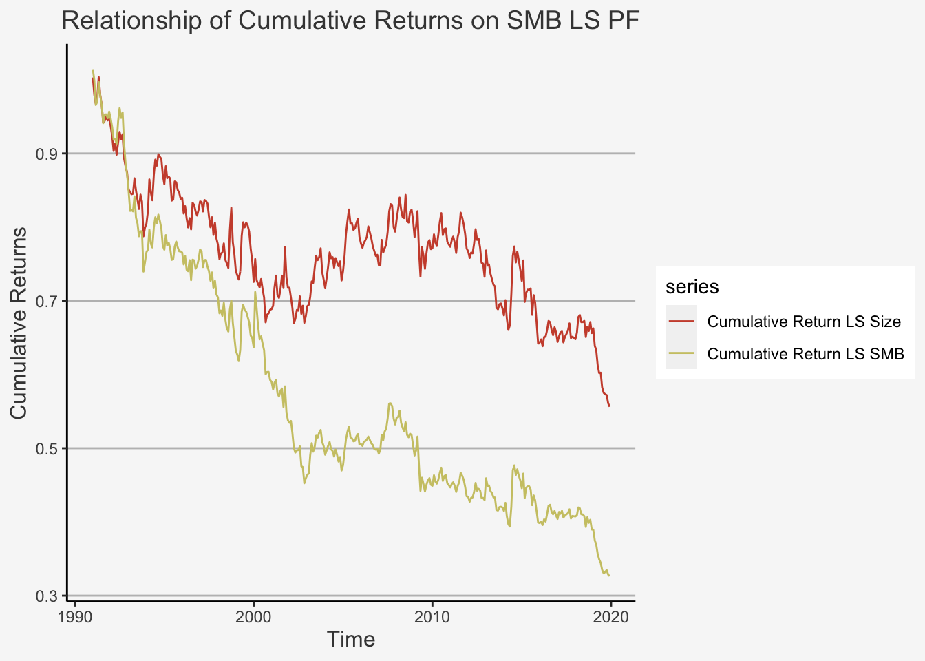
Great! We were able to construct the size factor based on both single- and double-sorting strategy. Interestingly, we observe that the Fama-French factor shows lower cumulative returns compared to the single-sorted factor. We can assess this observation analytically. For instance, we could deconstruct the factor again into its individual constituents. Note that the main difference between both was the inclusion of a value characteristic through a B2M ratio. Apparently, this inclusion decreases the cumulative returns quite considerably from the 2000’s on. Let’s visualise this as well:
# Calculate the Cumulative Product
Dates <- as.Date(dmy(Prices_Adj[,1][14:361]))
SMB_cp_components <- as.data.frame(cbind(Dates,
                              cumprod(1+EW_Returns_SL),
                              cumprod(1+EW_Returns_SM),
                              cumprod(1+EW_Returns_SH),
                              cumprod(1+EW_Returns_BL),
                              cumprod(1+EW_Returns_BM),
                              cumprod(1+EW_Returns_BH)))

# Create the xts object
SMB_cp_components_ts <- xts(x = SMB_cp_components[,-1], order.by = Dates)
names(SMB_cp_components_ts) <- c("Cumulative Return S/L", "Cumulative Return S/M", "Cumulative Return S/H", "Cumulative Return B/L", "Cumulative Return B/M", "Cumulative Return B/H")

# Create the plot for the double-sorted SMB Factor
SMB_plot_comp <- tidy(SMB_cp_components_ts) %>% ggplot(aes(x=index,y=value, color=series)) + geom_line() +
  scale_color_manual(values=c( "khaki3", "lightsteelblue3", "dodgerblue4", "tomato3", "violetred4", "darkorange2")) +
ylab("Cumulative Returns") + xlab("Time") + ggtitle("Relationship of Cumulative Returns on SMB LS PF - Components") +
labs(color='Factor Portfolios') +
  scale_colour_manual(values = c("lightsteelblue3","dodgerblue4", "darkorange2", "springgreen4", "violetred4", "goldenrod",  "khaki3")) +
  theme(plot.title= element_text(size=14, color="grey26",
  hjust=0.3,lineheight=2.4, margin=margin(15,0,15,0)),
  panel.background = element_rect(fill="#f7f7f7"),
  panel.grid.major.y = element_line(size = 0.5, linetype = "solid", color = "grey"),
  panel.grid.minor = element_blank(),
  panel.grid.major.x = element_blank(),
  plot.background = element_rect(fill="#f7f7f7", color = "#f7f7f7"),
  axis.title.y = element_text(color="grey26", size=12, margin=margin(0,10,0,10)),
  axis.title.x = element_text(color="grey26", size=12, margin=margin(10,0,10,0)),
  axis.line = element_line(color = "grey"))
## Scale for 'colour' is already present. Adding another scale for 'colour', which will replace the existing scale.SMB_plot_comp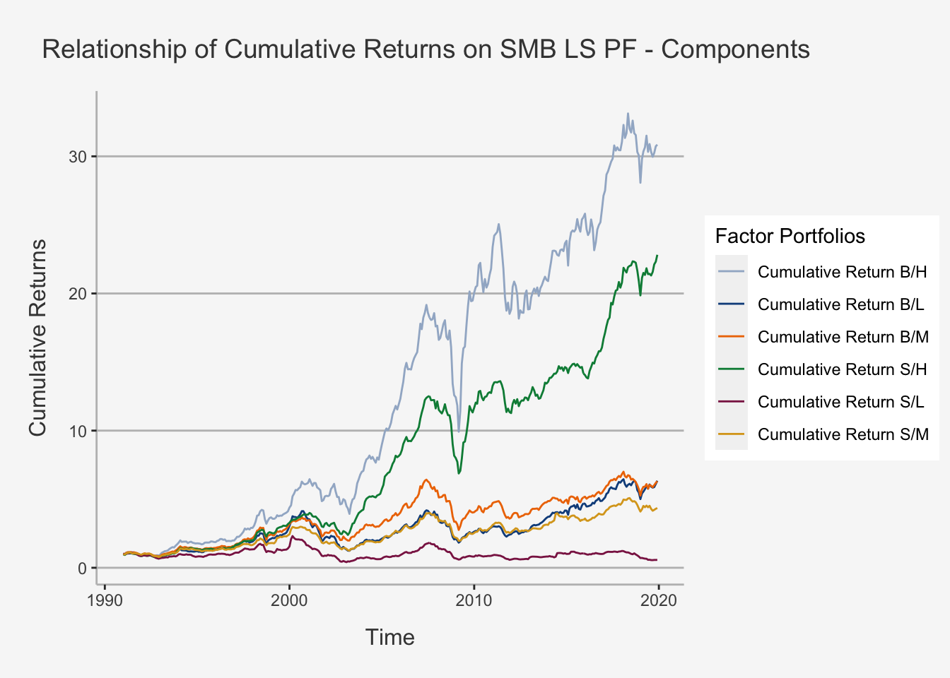
As we can observe, by distributing the average return into its constituents, we see that average returns are mainly driven by High B2M ratios. Furthermore, we can observe that, throughout all B2M characteristics, assets with larger than median market caps outperform their smaller counterparts. Given this mononous behaviour, it is apparent that the Size factor appears to no longer hold, at least when considering the last 30 years. Furthermore, it can be shown that, although the value factor is still valid, its magnitude depends on the market capitalisation of the securities under consideration, as higher B2M ratios outperform their lower counterparts only when we control for size (for instance, the second best performing portfolio is small and high, and it greatly outperforms the big and medium B2M ratio portfolio).
6.4.2.2 Fama-MacBeth Regression
We have seen the strength of the Fama-MacBeth (1973) procedure in assessing the ability of a covariate to explain movements in the cross-section of dependent returns during the application of the CAPM, where we were able to empirically prove that the movements of the market returns are unable to sufficiently explain the cross-sectional variation in asset returns. Given that the Market Return in the CAPM is nothing more than a factor itself, it is straight-forward to assume that we can replicate the procedure to include the factors under consideration.
However, since we are working with multiple factors, we need to generalise the formula we encountered in the previous chapter. As such, we first run a time-series regression of each asset’s excess return on the factors under consideration. That is, we run:
\[ r_{i,t} - r_{ft} = \alpha_i + \sum_{k=1}^K \beta_{i,k}f_k + \epsilon_{it} \]
whereas \(f_k\) is the k’th factor in the model.
Based on that, retrieve the factor loadings of each factor and perform a cross-sectional regression at each date, in which we regress the (excess) returns of each asset on the factor loadings. That is, we run:
\[ r_{i,t} - r_{ft} = \lambda_{i,0} + \sum_{k=1}^K \lambda_{i,k}\hat{\beta}_{i,k} + u_{it} \]
This is identical to what we have seen in the previous chapter. The only difference is now that we have multiple factors. This is represented by the sum sign. This means that we take factor loading 1 to k and run, at each date, the cross-section of asset returns on the asset returns.
Let’s recreate the FM (1973) approach and apply it to the SMB factor.
# Load the risk free rate as well as the Market Index
rf <- read.csv("~/Desktop/Master UZH/Data/A2_dataset_02_Ex_Session.txt", header = T, sep = "\t")
rf_sub <- subset(rf, (Date >= '1989-12-01') & (Date <= '2019-12-31'))
rf_ts <- xts(rf_sub[,-1], order.by = as.Date(dmy(Prices_Adj[,1])))
rf_ts_yearly <- rf_ts$SWISS.CONFEDERATION.BOND.1.YEAR...RED..YIELD / 100
rf_ts_monthly <- ((1 + rf_ts_yearly)^(1/12) - 1)['1991-01-01/2019-12-01']
colnames(rf_ts_monthly) <- "rf"

SMI <- read.csv("~/Desktop/Master UZH/Data/A2_dataset_03_Ex_Session.txt", header = T, sep = "\t")
SMI_sub <- subset(SMI, (Date >= '1989-12-01') & (Date <= '2019-12-31'))
SMI_ts <- xts(SMI_sub[,2], order.by = as.Date(dmy(Prices_Adj[,1])))
SMI_ts_ret <- Return.calculate(SMI_ts, method = "discrete")
Mkt_rf_SMI <- SMI_ts_ret['1991-01-01/2019-12-01'] - rf_ts_monthly['1991-01-01/2019-12-01']
colnames(Mkt_rf_SMI) <- "Index"

# Calculate the X and y variables for the regression
SPI_Index_ts <- merge.xts(Returns_Adj_ts['1991-01-01/2019-12-01'], rf_ts_monthly['1991-01-01/2019-12-01'], Mkt_rf_SMI['1991-01-01/2019-12-01'], SMB)

# First Pass Regression
for (i in names(SPI_Index_ts)[1:384]){
  col_name <- paste0(i)
  # Get the rolling window coefficients
  fit_roll_coefs <- summary(lm(SPI_Index_ts[,i] - SPI_Index_ts[,385] ~ SPI_Index_ts[,386] + SPI_Index_ts[,387]))$coefficients[2:3]

  if (i == 'NESN'){
    col_name_final <- col_name
    fit_roll_coefs_final <- fit_roll_coefs
  }
  else{
    col_name_final <- cbind(col_name_final, col_name)
    fit_roll_coefs_final <- cbind(fit_roll_coefs_final, fit_roll_coefs)
  }
}

# Set the column names
colnames(fit_roll_coefs_final) <- col_name_final

# Get the coefficients at each time period
beta_smb <- t(fit_roll_coefs_final)
colnames(beta_smb) <- c("MKT_RF", "SMB")

avg_ret <- t(SPI_Index_ts[,1:384])

# Bind them together
second_pass_data <- as.data.frame(cbind(beta_smb, avg_ret))

# Perform the second pass regression
factors = 2
models <- lapply(paste("`",names(second_pass_data[,2:350]) , "`", ' ~ MKT_RF + SMB', sep = ""),
function(f){ lm(as.formula(f), data = second_pass_data) %>%               # Call lm(.)
                         summary() %>%                                    # Gather the output
                         "$"(coef) %>%                                    # Keep only the coefs
                         data.frame() %>%                                 # Convert to dataframe
                         dplyr::select(Estimate)}                         # Keep only estimates
                 )
lambdas <- matrix(unlist(models), ncol = factors + 1, byrow = T) %>%
  data.frame()

colnames(lambdas) <- c("Constant", "MKT_RF", "SMB")

# We can now calculate the respective t statistics
T_Period <- length(names(second_pass_data[,2:350]))
average <- colMeans(lambdas, na.rm = T)
sd <- colStdevs(lambdas, na.rm = T)
se <- sd / sqrt(T_Period)
t_value <- average/se

# Create a final data frame
second_pass <- as.data.frame(cbind(average, se, t_value))
colnames(second_pass) <- c("Risk Premia Estimate", "Standard Error", "T-Stat")

round(second_pass, 4)
## Risk Premia Estimate Standard Error T-Stat
## Constant -0.0016 0.0045 -0.3631
## MKT_RF -0.0015 0.0021 -0.7409
## SMB 0.0063 0.0019 3.2394As we can see, the SMB factor is already quite successful in explaining the cross-sectional movements under consideration. However, note the following. If we leave the standard errors as is, we are highly likely to induce bias into the regression model. This is two-fold. Initially, we can refer to the usual issues in estimation accuracy based on the covariance structure of the assets under consideration. Note therein the heteroskedasticity and serial correlation assumptions we made in earlier chapters. Further, and even more worrisome, the factor loadings \(\hat{\beta}_{i,k}\) are estimates. This induces a bias arising from potential selection mistakes, or measurement error, as we have discussed. Usually, we need to further correct for this by applying different sorting or standard error correction techniques (to comprehend how, please refer to Shanken (1992)).
Lastly, we can visualise the behavior of the factor risk premia over time. Doing so, we will make use of the following visualisation.
# Here, we only take from the second row onwards
lambdas[2:nrow(lambdas),] %>%
  # We only select the factors of interet
  dplyr::select(MKT_RF, SMB) %>%
  # We then bind the columns such that we can gather them on the same x axis
  bind_cols(date = as.Date(names(second_pass_data[,3:350]))) %>%
  # We gather the factor and the lambda value based on each date
  gather(key = factor, value = lambda, -date) %>%
  # Here, we just create the ggplot
  ggplot(aes(x = date, y = lambda, color = factor)) +
  geom_line() + facet_grid(factor~.) +
  scale_color_manual(values=c("tomato3", "khaki3", "lightsteelblue3",
                              "dodgerblue4", "violetred4")) +
  theme_light()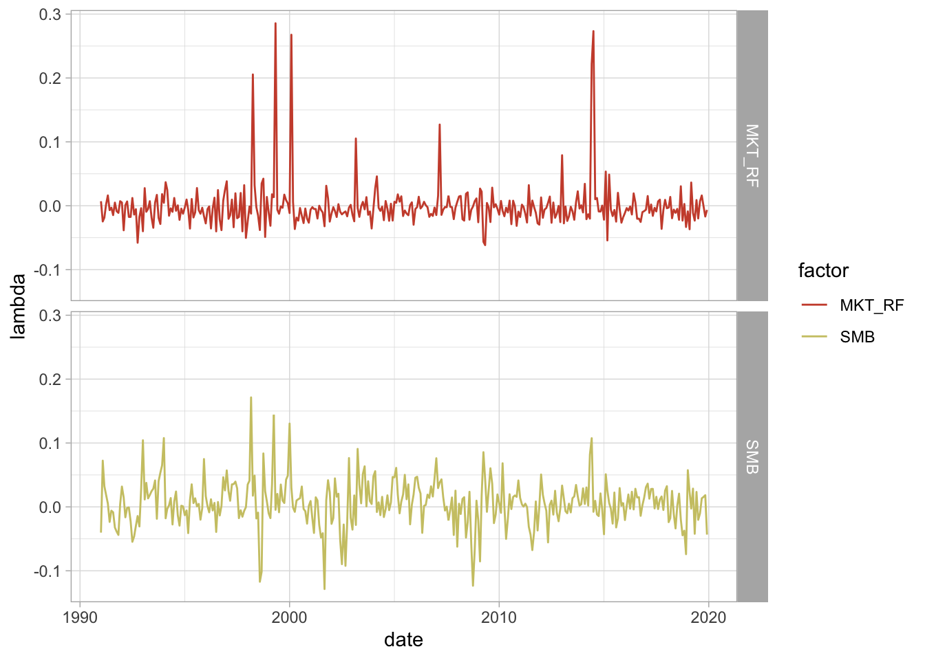
We can observe that both factors behave somewhat dependently on each other. That is, they could potentially represent collinearity issues. Both factors compensate in an unclear aggregate effect. This highlights the usefulness of penalized estimates, a machine learning technique that is used to reduce dimensionality of a regression framework. However, it is not the aim of this course to dive into this chapter (yet).
6.4.2.3 Factor Competition
As we stated, the main aim of of factors is to explain the cross-section of stock returns. However, as we have shown above, there is a potential that factors are moving simultaneously. In other words, it is likely that some factors are colinear to each other. As we understand it, collinearity is an issue because it absorbs variation of a given covariate, thereby making the estimates of interest redundant. If we have a variable which can be substantially represented by another variable within our model, then the resulting framework will induce variation which does not add explanatory power to the variation of the underlying variable of interest, but only noise. Without stating the theoretical concepts of this situation, this shares great similarities with the bias-and-variance issue usually encountered in machine learning applications. Therein, by introducing highly correlated variables, we add noise to the model which, subsequently, increases the standard errors and thus reduces the precision of the estimates. In addition, Guine (2021) states that, when asset managers decompose the performance of their returns into factors, overlaps (high absolute correlations) between factors yield exposures that are less interpretable; positive and negative exposures compensate each other in an uncomprehensible, or spurious, way.
They state a simple protocol to account for redundant factors, by running regressions of each factor against all others. That is, you run:
\[ f_{t,k} = \alpha_{k} + \sum_{j \neq k} \delta_{k,j}f_{t,j} + \epsilon_{t,k} \]
The authors state that the interesting metric is then the test statistic associated to the estimation of \(\alpha_k\).
- If \(\alpha_k\) is significantly different from zero, then the cross-section of (other) factors fails to explain exhaustively the average return of factor k.
- Otherwise, the return of the factor can be captured by exposures to the other factors and is thus redundant.
We will come back to this application once we encountered and retrieved more factors for the Swiss market.
6.5 Create your own factors: A step-by-step example
We have now leveraged the linear factor model and understand how to use these models in order to evaluate variation and detect anomalies. So far, the factors that we used were already pre-defined, meaning that we had the data already and “just” had to use the factor construction strategy discussed. However, without data there is not much to compute. Consequently, in the next part, we intend to bring you closer to the actual task of retrieving data needed to construct factor mimicking portfolios and then use the steps discussed above to coherently construct the factor(s) of interest. This will be quite helpful because it constitutes of all steps necessary to construct, apply and interpret factors (and thus resembles the day to day work within factor setting asset management companies).
However, a major difference to all external asset managers is that we intend not to take too long in order to retrieve the data at hand :-). As such, we will again introduce the field of the relational database computing. We have elaborated the SQL coding approach to retrieve data from a relational database. However, we now enhanced the function which automates the entire process for us such that we can now get data from CRSP, Compustat as well as Thomson Reuters / Datastream. The latter is important because it allows us to access the worldscope data base, which offers the largeest consortium of company financials as well as security characteristics for Non-US stocks.
6.5.1 Setting up the WRDS proxy
The function for WRDS Database Query is the following. Again, you don’t need to know the function by heart. However, there are still multiple databases which this function cannot (yet) retrieve. Thus, if you feel like something is missing, try modifying the function and see if you are able to get what you need. Any help is certainly greatly appreciated!
# Create a function to automate the data retrieval jobs on SQL
dataset_a = NULL
dataset_b = NULL
dataset_sql = NULL

datafmt = NULL
consol = NULL
indfmt = NULL
sic = NULL
gvkey = NULL
tic= NULL
cusip= NULL
isin = NULL

filters_list= NULL
filters_list_final= NULL
filters_list_tweaked= NULL
filters_list_tweaked_final= NULL

query_sql <-
  function(dataset_a, dataset_b, column_a, column_b, column_sql, start, end, datafmt, consol, indfmt, sic, gvkey, tic, cusip, isin, multi_function = TRUE, reuters_ds = FALSE){

    if (reuters_ds == FALSE){

      if (!is.null(column_a)) {
      for (i in 1:length(column_a)) {
      column_a[i] = paste("a.", column_a[i], sep = "")
      column_filter_a = paste(column_a, collapse = ',')
      }
    }
    else {
      columns_filter_a = ""
    }

    if (!is.null(column_b)) {
      for (i in 1:length(column_b)) {
      column_b[i] = paste("b.", column_b[i], sep = "")
      column_filter_b = paste(column_b, collapse = ',')
      }
    }
    else {
      columns_filter_b = ""
    }

    if (!is.null(column_sql)) {
      for (i in 1:length(column_sql)) {
      column_sql[i] = paste("b.", column_sql[i], sep = "")
      column_filter_sql = paste(column_sql, collapse = ',')
      }
    }
    else {
      columns_filter_sql = ""
    }

    if (!is.null(start) & !is.null(end)){
      date_filter = paste("a.datadate BETWEEN '", start, "' AND '", end, "'")
    }

    sic_filter = NULL
    if (!is.null(sic)) {
      for (i in 1:length(sic)) {
      sic[i] = paste("'", sic[i], "'", sep = "")
      sic_filter = paste("a.sic IN (", paste(sic, collapse = ','), ")")
      }
    }

    gvkey_filter = NULL
    if (!is.null(gvkey)) {
      for (i in 1:length(gvkey)) {
      gvkey[i] = paste("'", gvkey[i], "'", sep = "")
      gvkey_filter = paste("a.gvkey IN (", paste(gvkey, collapse = ','), ")")
      }
    }

    tic_filter = NULL
    if (!is.null(tic)) {
      for (i in 1:length(tic)) {
      tic[i] = paste("'", tic[i], "'", sep = "")
      tic_filter = paste("a.tic IN (", paste(tic, collapse = ','), ")")
      }
    }

    cusip_filter = NULL
    if (!is.null(cusip)) {
      for (i in 1:length(cusip)) {
      cusip[i] = paste("'", cusip[i], "'", sep = "")
      cusip_filter = paste("a.cusip IN (", paste(cusip, collapse = ','), ")")
      }
    }

    if (!is.null(datafmt)) {
      for (i in 1:length(datafmt)) {
      datafmt[i] = paste("a.datafmt =  '", datafmt[i], "'", sep = "")
      datafmt_filter = paste(datafmt, collapse = ',')

      }
    }

    if (!is.null(consol)) {
      for (i in 1:length(consol)) {
      consol[i] = paste("a.consol =  '", consol[i], "'", sep = "")
      consol_filter = paste(consol, collapse = ',')

      }
    }

    if (!is.null(indfmt)) {
      for (i in 1:length(indfmt)) {
      indfmt[i] = paste("a.indfmt =  '", indfmt[i], "'", sep = "")
      indfmt_filter = paste(indfmt, collapse = ',')

      }
    }

    filters = c(date_filter, cusip_filter, tic_filter, gvkey_filter, sic_filter, datafmt_filter, consol_filter, indfmt_filter)

    for (i in 1:length(filters)){
      if (!is.null(filters[i])){
        filters_list[i] = paste(filters[i], sep = "")
        filters_list_final = paste(" WHERE ", paste(filters_list, collapse = " AND "))
      }
    }

    filters_tweaked = c(date_filter, cusip_filter, tic_filter, gvkey_filter, sic_filter)

    if (!is.null(filters_tweaked[i])){
       for (i in 1:length(filters_tweaked)){
        filters_list_tweaked[i] = paste(filters_tweaked[i], sep = "")
        filters_list_tweaked_final = paste(" WHERE ", paste(filters_list_tweaked, collapse = " AND "))
      }
    }

    if (multi_function == TRUE){
      sql = (paste("SELECT ",
                   column_filter_a,
                   ", ", column_filter_b,
                   " FROM  ", dataset_a, " a",
                   " inner join ", dataset_b, " b",
                   " on ", column_a[1], " = ", column_sql[1],
                   " and ", column_a[2], " = ", column_sql[2],
                   " and ", column_a[3], " = ", column_sql[3],
                   filters_list_final))
    }

    else {
      sql = (paste("SELECT ",
                   column_filter_a,
                   " FROM  ", dataset_a, " a",
                   filters_list_tweaked_final))
    }

  }

  else {
      if (!is.null(column_a)) {
        for (i in 1:length(column_a)) {
        column_a[i] = paste("a.", column_a[i], sep = "")
        column_filter_a = paste(column_a, collapse = ',')
        }
      }
      else {
        columns_filter_a = ""
      }

      if (!is.null(column_b)) {
        for (i in 1:length(column_b)) {
        column_b[i] = paste("b.", column_b[i], sep = "")
        column_filter_b = paste(column_b, collapse = ',')
        }
      }
      else {
        columns_filter_b = ""
      }

      if (!is.null(column_sql)) {
        for (i in 1:length(column_sql)) {
        column_sql[i] = paste("b.", column_sql[i], sep = "")
        column_filter_sql = paste(column_sql, collapse = ',')
        }
      }
      else {
        columns_filter_sql = ""
      }

      if (!is.null(start) & !is.null(end)){
        date_filter = paste("a.year_ BETWEEN '", start, "' AND '", end, "'")
      }

      sic_filter = NULL
      if (!is.null(sic)) {
        for (i in 1:length(sic)) {
        sic[i] = paste("'", sic[i], "'", sep = "")
        sic_filter = paste("a.sic IN (", paste(sic, collapse = ','), ")")
        }
      }

      gvkey_filter = NULL
      if (!is.null(gvkey)) {
        for (i in 1:length(gvkey)) {
        gvkey[i] = paste("'", gvkey[i], "'", sep = "")
        gvkey_filter = paste("a.gvkey IN (", paste(gvkey, collapse = ','), ")")
        }
      }

      tic_filter = NULL
      if (!is.null(tic)) {
        for (i in 1:length(tic)) {
        tic[i] = paste("'", tic[i], "'", sep = "")
        tic_filter = paste("a.item5601 IN (", paste(tic, collapse = ','), ")")
        }
      }

      cusip_filter = NULL
      if (!is.null(cusip)) {
        for (i in 1:length(cusip)) {
        cusip[i] = paste("'", cusip[i], "'", sep = "")
        cusip_filter = paste("a.item6004 IN (", paste(cusip, collapse = ','), ")")
        }
      }

      isin_filter = NULL
      if (!is.null(isin)) {
        for (i in 1:length(isin)) {
        isin[i] = paste("'", isin[i], "'", sep = "")
        isin_filter = paste("a.item6008 IN (", paste(isin, collapse = ','), ")")
        }
      }


      filters = c(date_filter, cusip_filter, tic_filter, gvkey_filter, sic_filter, isin_filter)

      for (i in 1:length(filters)){
        if (!is.null(filters[i])){
          filters_list[i] = paste(filters[i], sep = "")
          filters_list_final = paste(" WHERE ", paste(filters_list, collapse = " AND "))
        }
      }

      filters_tweaked = c(date_filter, cusip_filter, tic_filter, gvkey_filter, sic_filter, isin_filter)

      if (!is.null(filters_tweaked[i])){
         for (i in 1:length(filters_tweaked)){
          filters_list_tweaked[i] = paste(filters_tweaked[i], sep = "")
          filters_list_tweaked_final = paste(" WHERE ", paste(filters_list_tweaked, collapse = " AND "))
        }
      }

      if (multi_function == TRUE){
        sql = (paste("SELECT ",
                     column_filter_a,
                     ", ", column_filter_b,
                     " FROM  ", dataset_a, " a",
                     " inner join ", dataset_b, " b",
                     " on ", column_a[1], " = ", column_sql[1],
                     " and ", column_a[2], " = ", column_sql[2],
                     " and ", column_a[3], " = ", column_sql[3],
                     filters_list_final))
      }

      else {
        sql = (paste("SELECT ",
                     column_filter_a,
                     " FROM  ", dataset_a, " a",
                     filters_list_tweaked_final))
      }
    }

  }
Note that we will retrieve the data needed from the WRDS services. In order to use their services, we need to log onto their system. This can be done again by using the command below.
# Open the connection
wrds <- dbConnect(Postgres(),
                  host='wrds-pgdata.wharton.upenn.edu',
                  port=9737,
                  dbname='wrds',
                  sslmode='require',
                  user='gostlow',
                  password = "climaterisk8K")
Once the credentials are valid, we can access the database and start retrieving the data we require.
6.5.2 Factors of interest
Having established a connection to the WRDS services, the next question is which factors we want to create ourselves. In order to do so, we will focus at the most commonly known and publicly cited anomaly factors currently present. These include:
- Size (Small Minus Big (SMB))
- Value (High Minus Low (HML))
- Momentum (Winners Minus Losers (WML))
- Profitability (Robust Minus Weak (RMW))
- Investment (Conservative Minus Aggressive (CMA))
- Low Risk (Betting Against Beta (BAB))
We already know how to calculate the Size factor. However, for the remaining factors, we still need to define the common framework of construction.
The Value factor is constructed by retrieving data on the Book to Market Ratio (B2M). The formula is:
\[ \text{B2M}_t = \frac{\text{Book-Equity}_{t-6}}{\text{Market Cap}_t} \]
Using this formula, at each date t, we go long in assets with a high Book-to-Market Ratio and Short in assets with a low Book-to-Market ratio. Therein, we define High and Low as the 30th and 70th percentile of the distribution, respectively. The respective indicator on High and Low B2M Ratios is then interacted with the indicator on small or large cap firms, whereas we use the median value as cut-off for the company size.
The factor is then constructed using the following formula:
\[ \text{HML}_t = 1/2 * (SH_t + BH_t) - 1/2*(SL_t + BL_t) \]
whereas \(SH_t\) is the equal- or value-weighted return of small (below or at median) market cap and high B2M (above 70th percentile) stocks, \(BH_t\) is the return of Big and High B2M securities and \(SL_t\) as well as \(BL_t\) are their low B2M counterparts.
The Momentum factor is constructed by retrieving the data on Adjusted Stock Prices. The formula is:
\[ \text{Momentum}_t = \frac{\text{Prices Adjusted}_{t-1} - \text{Prices Adjusted}_{t-12}}{\text{Prices Adjusted}_{t-12}} \]
Using this formula, at each date t, we go long in assets with a high Past Adjusted return and Short in assets with a low Past Adjusted return. Therein, we define High and Low again as the 30th and 70th percentile of the distribution, respectively. The respective indicator on High and Low Past Return Adjusted Ratios is then interacted with the indicator on small or large cap firms, whereas we use the median value as cut-off for the company size.
The factor is then constructed using the following formula:
\[ \text{WML}_t = 1/2 * (SW_t + BW_t) - 1/2*(SL_t + BL_t) \]
whereas \(SW_t\) is the equal- or value-weighted return of small (below or at median) market cap and return winner (above 70th percentile) stocks, \(BW_t\) is the return of Big and return winner securities and \(SL_t\) as well as \(BL_t\) are their return loser counterparts.
The Profitability factor is constructed by retrieving the data on revenues, cost, expenses as well as book equity. The formula is:
\[ \text{Profitability}_t = \frac{\text{Operating Income}_{t} - \text{COGS}_{t} - \text{SGAE}_{t} - \text{Interest Expenses}_{t} }{\text{Total Book Equity}_{t}} \]
whereas Operating Income is just the total income from operations, COGS are the Costs of Goods Sold, SGAE are Selling, General and Administrative Expenses and Total Book Equity is the Equity of the Balance Sheet. Note that COGS and SGAE are also sometimes referred to as Operating Expenses (although they are not identical they match quite well so for calculation purposes it should not depend too greatly on which accounting numbers you take).
Using this formula, at each date t, we go long in assets with a high Profitability and Short in assets with a low Profitability. Therein, we define High and Low again as the 30th and 70th percentile of the distribution, respectively. The respective indicator on High and Low Past Return Adjusted Ratios is then interacted with the indicator on small or large cap firms, whereas we use the median value as cut-off for the company size.
The factor is then constructed using the following formula:
\[ \text{RMW}_t = 1/2 * (SR_t + BR_t) - 1/2*(SW_t + BW_t) \]
whereas \(SR_t\) is the equal- or value-weighted return of small (below or at median) market cap and robust (above 70th percentile) stocks, \(BR_t\) is the return of Big and robust securities and \(SW_t\) as well as \(BW_t\) are their rprofitability weak counterparts.
The Investment factor is constructed by retrieving the data on total assets. The formula is:
\[ \text{Investment}_t = \frac{\text{Total Assets}_{t} - \text{Total Assets}_{t-1}}{\text{Total Assets}_{t-1}} \]
Aggressive firms are those that experience the largest growth in assets. Using this formula, at each date t, we go long in assets with a high Asset growth and Short in assets with a low Asset growth. Therein, we define High and Low again as the 30th and 70th percentile of the distribution, respectively. The respective indicator on High and Low Past Return Adjusted Ratios is then interacted with the indicator on small or large cap firms, whereas we use the median value as cut-off for the company size.
The factor is then constructed using the following formula:
\[ \text{CMA}_t = 1/2 * (SC_t + BC_t) - 1/2*(SA_t + BA_t) \]
whereas \(SC_t\) is the equal- or value-weighted return of small (below or at median) market cap and conservative (below 30th percentile) stocks, \(BC_t\) is the return of Big and conservative securities and \(SW_t\) as well as \(BW_t\) are their asset growth aggressive counterparts.
Lastly, the Betting Against Beta factor is constructed in a somewhat advanced manner. We follow the approach by Frazzini and Pedersen (2014) here and construct the factor by running rolling regressions of the excess returns on market excess returns. However, we will not directly run the regressions. Rather, we will calculate the following formula for each beta at date t:
\[ \hat{\beta}_{TS}= \hat{\rho}\cdot \frac{\hat{\sigma}_i}{\hat{\sigma}_M} \]
whereas \(\hat{\sigma}_i\) and \(\hat{\sigma}_i\) are the estimated volatilities for the stock and the market and \(\hat{\rho}\) is their estimated their correlation. They use a one-year rolling standard deviation to estimate volatility as well as a five-year horizon for the correlation.
Lastly, the authors reduce the influence of outliers by following Vasicek (1973) and construct a shrinkage of the time series estimate of beta towards 1 by running:
\[ \hat{\beta}_{i} = 0.4\cdot \hat{\beta}_{TS} + 0.6 \cdot 1 \]
Having constructed the beta estimates, they rank the betas and go long in assets with a below median beta value and short in assets with an above median beta value.
Then, in each portfolio, securities are weighted by the ranked betas (i.e., lower-beta securities have larger weights in the low-beta portfolio and higher-beta securities have larger weights in the high-beta portfolio). To put it more formally, we have that \(z_i = rank(\hat{\beta}_{it})\) and \(\bar{z} = \frac{1}{n}\sum_{i=1}^N z_i\), whereas \(z_i\) indicates the rank of the i’th beta and \(\bar{z}\) is the average rank, where n is the number of securities.
Based on this, the portfolio weights are constructed as:
\[ w_{it} = k(z_{it} - \bar{z}_t) \]
whereas \(k = \frac{2}{\sum_{i=1}^N |z_i - z|}\) is a normalisation constant. Based on these weights, we can finally construct the BAB factor as:
\[ \text{BAB}_t = \frac{1}{\sum_{i=1}^N\beta_{it}^Lw_{it}^L}(\sum_{i=1}^N r_{i,t+1}^Lw_{it}^L - r_f) - \frac{1}{\sum_{i=1}^N\beta_{it}^Hw_{it}^H}(\sum_{i=1}^N r_{i,t+1}^Hw_{it}^H - r_f) \]
For all the factors, it is important to understand that they need to be lagged by one period to avoid any look-ahead bias.
6.5.3 Get the data to construct the factors
We now proceed by retrieving the data from the datastream services. Therein, we will need to fetch two distinct types of data. The company stock characteristics which are taken from the datastream equitites database, as well as the company fundamanetals characteristics through the worldscope database. Note that, to show you how to retrieve the data in multiple ways, we decided to retrieve the data on stock characteristics manually while using the function to retrieve the data on company fundamentals. The exact composition of the services of Datastream worldscope as well as the respective names can be found on the WRDS homepage, whereas you can find the compositon of the services of Datastream equities here. For our use, we will need the Daily Stock File (wrds_ds2dsf) from the equities database as well as the Fundamentals Annually (wrds_ws_funda) as well as the Stock Data (wrds_ws_stock) tables of the worldscope database.
The variables that we retrieve from the equities database are given below:
- adjclose: Adjusted Close price (Used for: MOM)
- close: Unadjusted Close price (Used for: SMB, HML)
- volume: Volume of traded shares
- numshrs: Number of shares outstanding (Used for: SMB, HML)
Further, we need some identifiers to assure that we only take the Swiss companies under consideration:
- dscode: Code identifier for the stocks of TR
- marketdate: Date of the observation
- currency: Currency the company is traded in
- region: Region of company’s main location
- isin: ISIN number
- ticker: Ticker
- dslocalcode: Local code (combination of ISIN and Ticker based on TR)
While the names for the equities database are quite straight-forward to interpret, the variable names of the worldscope database are presented in “items”, whereas each item is associated with a different accounting number. These are indicated below:
item3501: Common Equity (= Book Value. Used for: HML, RMW. From wrds_ws_funda)
item2999: Total Assets (Used for: HML, CMA. From: wrds_ws_funda)
item3351: Total Liabilities (Used for: HML. From: wrds_ws_funda)
item1001: Net Sales or Revenues (Used for: RMW. From: wrds_ws_funda)
item1051: COGS excl depreciation (Used for: RMW. From: wrds_ws_funda)
item1101: SGA (Used for: RMW, From wrds_ws_funda)
item1100: Gross Income
item1249: Operating Expenses
item1251: Interest Expense on Debt
Moreover, we need data on the date and sequence codes
- year_: Year of observation
- seq: Sequential code
- code: Company code from TR
- item5350: Fiscal Period End date (Used to identify at which date the company had its annual closing. Based on this date, the 12 previous periods will obtain the same accouting numbers when upsampling from annual to monthly observations - e.g. if a company has its reported closing on the 31st of March, then the respective accounting number must be replicated for the subsequent 12 periods in order to base portfolios on the characteristic).
Further, we need to define for which companies we require the data at hand. As it was with the data in CRSP and Compustat, we can enter a search query by providing security information based on (I) Stock Ticker (II) ISIN Number (III) CUSIP Number (IV) IBES identifier. However, we always advise you to use CUSIP numbers whenever possible, as these are the truly unique identifiers that can be used to source multiple databases at once. In our case, these are the following items:
- item5601: Ticker Symbol
- item6008: ISIN
- item6004: CUSIP
- item6038: IBES
For the use case here, we have a comprehensive ticker dataset with the companies that we previously used for earlier exercises. We will use this as identifier for our securities.
6.5.3.1 Fetch the Swiss Data for Stock Characteristics through datastream equitites
# Get the stock market data (shares outstanding, adjusted and unadjusted stock prices, volume of trades)
res <- dbSendQuery(wrds, "select  a.dscode, a.marketdate,a.adjclose,a.close,a.volume, a.numshrs, a.ri, a.currency, a.region,
                          b.isin, b.ticker, b.dslocalcode
                          from  tr_ds_equities.wrds_ds2dsf a
                          left join tr_ds_equities.wrds_ds_names b
                          on a.dscode = b.dscode
                          where a.marketdate BETWEEN '1990-01-01' and '2021-12-31' AND a.region = 'CH'")

data_2 <- dbFetch(res)

# Split the ISIN into two parts
# This is done to identify Swiss companies with the characteristic "CH" in front of the ISIN number
CH_data <- data_2 %>%
  mutate(country = substr(data_2$isin,1,2)) %>%
  subset(country == "CH" & currency == "CHF")

# Get the calender week
CH_data <- CH_data %>% mutate(Cal_Week = lubridate::week(marketdate))

# Expand the date
CH_data_stock <- separate(CH_data, "marketdate", c("Year", "Month", "Day"), sep = "-")

# Delete duplicated rows
CH_data_stock <- CH_data_stock[!duplicated(CH_data_stock[c("Year", "Month", "Day", 'ticker', 'dscode')]),]

# Monthly Data: Get only the last date of each month
CH_data_stock_monthly <-  CH_data_stock %>%
  # Group by each year-month and company
  group_by(dscode, Year, Month) %>%
  # Only get the maximum day value (the last day of each month per company and year)
  filter(Day == max(Day)) %>%
  # Recreate the actual last day date
  mutate(Date_actual = as.Date(paste(Year,Month,Day,sep="-")),
         # Since this is only the last observed date, we need to transform them into the last date of each month (e.g. if last observed day was 2000-06-28 we
         # need to transform this to 2000-06-30 to match the relationship afterwards)
         Date_t = lubridate::ceiling_date(Date_actual, "month") - 1) %>%
  ungroup() %>%
  select(Date_t, ticker, isin, adjclose, close, numshrs)

# Weekly Data: Get only the last date of each week (same logic as above, but this time with weeks and not months)
CH_data_stock_weekly <- CH_data_stock %>%
  group_by(dscode, Year, Month, Cal_Week) %>%
  filter(Day == max(Day)) %>%
  mutate(Date_t = as.Date(paste(Year,Month,Day,sep="-"))) %>%
  ungroup() %>%
  select(Date_t, ticker, isin, adjclose, close, numshrs)
6.5.3.2 Fetch the Swiss data for company fundamanetals characteristics through worldscope
# First, we define the ticker symbol
tic <- unique(CH_data_stock_monthly$ticker)

# Then, we define the variables to be retrieved
column_a <- list('year_', 'seq', 'code', 'item5350', # Date and sequence codes
                 "item5601", "item6008", "item6004", "item6038", # The identifiers
                 "item3501", "item2999", "item3351", # Common Equity, Total Assets, Total Liabs
                 "item1001", "item1051", "item1101", "item1100", "item1249", "item1251") # Total Revenue, COGS, SGA, Gross Income, Operating Exp, Interest Exp)


# This is to connect the both databases without duplicating their output in the end
column_sql = list('year_', 'seq', 'code')

# This is the second database, used for the keys from the securities monthly list
column_b = list('item8001', 'item8004') # Market Cap, Market Cap Public

# Get the quarterly data on company financials
query = query_sql(dataset_a = "tr_worldscope.wrds_ws_funda",
                  dataset_b = "tr_worldscope.wrds_ws_stock",
                  multi_function = F,
                  reuters_ds = T,
                  column_a = column_a,
                  column_b = column_b,
                  column_sql = column_sql,
                  gvkey = gvkey,
                  sic = sic,
                  tic = tic,
                  cusip = cusip,
                  isin = isin,
                  datafmt = NULL,
                  consol = 'C',
                  indfmt = 'INDL',
                  start = '1990',
                  end = '2022')

res <- dbSendQuery(wrds, query)
## Warning in result_create(conn@ptr, statement, immediate): Closing open result set, cancelling previous querydata <- dbFetch(res)
colnames(data) <- c('Year_t', 'Seq', 'Code', "Fiscal_Period_End_Date",
"Ticker", "ISIN", "CUSIP", "IBES",
"Total_Eq_t", "Total_Assets_t", "Total_Liab_t",
"Revenue_Tot_t", "COGS_t", "SGA_t", "Gross_Inc_t", "Operating_Exp_t", "Interest_Exp_t")
# Split the ISIN into two parts
CH_data_fund <- data %>%
mutate(country = substr(data$ISIN,1,2)) %>%
subset(country == "CH")
# Remove duplicated observations based on the Code and Year combination
CH_data_fund <- CH_data_fund[!duplicated(CH_data_fund[c('Year_t', 'Code')]),]
CH_data_fund <- separate(CH_data_fund, "Fiscal_Period_End_Date", c("Year_Fiscal_Period_End", "Month_Fiscal_Period_End", "Day_Fiscal_Period_End"), sep = "-")
# Create the monthly dataset
CH_data_fund_monthly <- CH_data_fund %>%
mutate(Dupl_Dummy = ifelse(!is.na(Total_Assets_t) | !is.na(Total_Liab_t), 1, 0)) %>%
subset(Dupl_Dummy == 1) %>%
group_by(Year_t, Code) %>%
slice(rep(1:n(), first(12))) %>%
# Expand the data from yearly to monthly while accounting for different fiscal period end dates
mutate(Month_t = ifelse(Month_Fiscal_Period_End == "01",
c(02, 03, 04, 05, 06, 07, 08, 09, 10, 11, 12, 01),
ifelse(Month_Fiscal_Period_End == "03",
c(04, 05, 06, 07, 08, 09, 10, 11, 12, 01, 02, 03),
ifelse(Month_Fiscal_Period_End == "04",
c(05, 06, 07, 08, 09, 10, 11, 12, 01, 02, 03, 04),
ifelse(Month_Fiscal_Period_End == "05",
c(06, 07, 08, 09, 10, 11, 12, 01, 02, 03, 04, 05),
ifelse(Month_Fiscal_Period_End == "06",
c(07, 08, 09, 10, 11, 12, 01, 02, 03, 04, 05, 06),
ifelse(Month_Fiscal_Period_End == "07",
c(08, 09, 10, 11, 12, 01, 02, 03, 04, 05, 06, 07),
ifelse(Month_Fiscal_Period_End == "08",
c(09, 10, 11, 12, 01, 02, 03, 04, 05, 06, 07, 08),
ifelse(Month_Fiscal_Period_End == "09",
c(10, 11, 12, 01, 02, 03, 04, 05, 06, 07, 08, 09),
ifelse(Month_Fiscal_Period_End == "10",
c(11, 12, 01, 02, 03, 04, 05, 06, 07, 08, 09, 10),
ifelse(Month_Fiscal_Period_End == "11",
c(12, 01, 02, 03, 04, 05, 06, 07, 08, 09, 10, 11),
c(01, 02, 03, 04, 05, 06, 07, 08, 09, 10, 11, 12)
)
)
)
)
)
)
)
)
)
),
Day_t = c(01, 01, 01, 01, 01, 01, 01, 01, 01, 01, 01, 01),
# Create for each month the starting period
Start_Date_t = as.Date(paste(Year_t,Month_t,Day_t,sep="-")),
# And also the last day of the month -> assign as Date column since we only work with last day of month values (They are the same anyways)
Date_t = lubridate::ceiling_date(Start_Date_t, "month") - 1
) %>%
ungroup() %>%
# Select only the variables of interest
select(Date_t, Ticker, ISIN, Total_Assets_t, Total_Liab_t, Gross_Inc_t, Operating_Exp_t, Interest_Exp_t, Total_Eq_t)
colnames(CH_data_stock_monthly) = c("Date_t", "Ticker", "ISIN", "Adj_Close", "Close", "Num_Shares")6.5.3.3 Export the monthly and weekly datasets
# Create a dataframe which incorporates all data
CH_data_total_monthly <- left_join(CH_data_stock_monthly, CH_data_fund_monthly,
              by = c("Ticker" = "Ticker", "Date_t" = "Date_t"))

write.csv(CH_data_total_monthly, "~/Desktop/CH_data_total_monthly.csv", row.names = FALSE)

# Write the weekly csv for stocks
write.csv(CH_data_stock_weekly, "~/Desktop/CH_data_stock_weekly.csv", row.names = FALSE)
6.5.4 Portfolio Sorts for different factors
We first deploy the portfolio sorts strategy to determine the behaviour of percentile distributed portfolios based on the characteristic of interest. Therein, we will create decile portfolios which are sorted based on the factors of interest.
However, before we start, we need to clarify the following. Previously, we used a specific approach to construct factors. This approach is also known as wide format approach, because we use a wide formatted dataframe in order to calculate the factor returns. Remember that a wide formatted dataframe means that each column shows the data of one specific characteristic for one specific company. Thus, if you have 300 companies for 10 years on a yearly basis, then the dataframe will have 300 columns and 10 rows. This implies that we need multiple dataframes to construct multiple factors.
The other method is called the long format approach. This is because we use a long formatted dataframe. As opposed to a wide formatted dataframe, long formats are constructed such that, in each column, we have a specific accounting number. In the other two columns, we then have the respective observational period as well as the company identifier for the respective accounting measure. For instance, if you have 3 specific measures (let’s say Total Equity, Net Income as well as Turnover) for 300 companies and 10 years, then you have a dataframe consisting of 5 columns and 3000 rows (300 companies à 10 years). This implies that we only need one dataframe to construct multiple factors.
We showed you the wide format approach previously because, although it appears to be computationally more complex, it actually shows all the specific steps we make when constructing factors. That is, you can trace pretty much each step back to its direct predecessor and thereby comprehend more easily how the code operates.
Despite this, we now introduce the long format approach. Although it does not document each operation directly, the main advantage is that it is computationally less expensive. As such, we can retrieve the results with less code and running time.
However, for one specific factor, the Jegadeesh Momentum factor, we still create the factors in both forms. This is to show you the main concepts in both ways. Especially, we want to highlight some differences in the sorting strategy that R follows which can potentially lead to slightly different results. In general, sorting is still a highly debated field with multiple different possibilities that statistics programs offer. When we use a pre-defined sorting function, we are likely to obtain different sorts compared to using a customised (own created) sorting procedure. Although this can lead to different results, it shows an additional, important caveat for scientific work. That is, we need to be clear and precise in formulating our assumptions even in more technical and less central areas of the work at hand.
6.5.4.1 Jegadeesh and Titman Momentum Factor
This is the replication of the Jegadeesh and Titman Momentum factor. Therein, we will construct the factors in both a wide and long format to show you the differences that the choice of the sorting function can have on the final performance of our portfolios. Note that this is not the same Momentum factor as we will cover in the last assignment and, thus, it cannot be copied to calculate the momentum factor.
6.5.4.1.1 Wide-format factor construction
# Let's run the experiment for the reduced data frame
tic_sub <- unique(names(read.csv("~/Desktop/Master UZH/Data/A4_dataset_04_Ex_Session.txt", header = T, sep = "\t")))
# Get 347 companies
CH_data_total_monthly <- read.csv("~/Desktop/CH_data_total_monthly.csv", header = T, sep = ",")
# Create a wide data frame
CH_data_total_monthly_clean <- CH_data_total_monthly[!duplicated(CH_data_total_monthly[c("Date_t", "Ticker")]),]

CH_data_total_monthly_clean <- CH_data_total_monthly_clean %>%
  subset(Ticker %in% tic_sub) %>%
  select(Date_t, Ticker, Adj_Close)

CH_data_total_monthly_clean_wide <- CH_data_total_monthly_clean %>% na.omit() %>% spread(key = Ticker, value = Adj_Close)

# Create time series object
CH_data_total_monthly_clean_wide_ts <- xts(CH_data_total_monthly_clean_wide[,-1], order.by = as.Date(CH_data_total_monthly_clean_wide$Date_t))

# Calculate Returns
CH_data_total_monthly_wide_ret_ts <- Return.calculate(CH_data_total_monthly_clean_wide_ts, "discrete")

# Cut the 5% most extreme returns
extreme_cutoff <- matrixStats::rowQuantiles(as.matrix(CH_data_total_monthly_wide_ret_ts), probs = 0.999, na.rm = T)


for (i in names(CH_data_total_monthly_wide_ret_ts)){
  extreme <- ifelse(CH_data_total_monthly_wide_ret_ts[,i] <= extreme_cutoff, 1, NA)

  if (i == "ABBN"){
    extreme_final <- extreme
  }
  else {
    extreme_final <- cbind(extreme_final, extreme)
  }
}

CH_data_total_monthly_wide_ret_ts <- CH_data_total_monthly_wide_ret_ts*extreme_final

# Calculate Cumulative Returns
for (i in names(CH_data_total_monthly_wide_ret_ts)){
  col_name <- paste0(i)
  Log_Ret_Adj = log(1+CH_data_total_monthly_wide_ret_ts[,i])
  Sum_Ret = roll_sum(Log_Ret_Adj, 6)
  Cum_Ret = exp(Sum_Ret) - 1

  if (i == "ABBN"){
    Cum_Ret_final <- Cum_Ret
  }
  else{
    Cum_Ret_final <- cbind(Cum_Ret_final, Cum_Ret)
  }
}

one_to_ten <- seq(1,10,1)

for (i in one_to_ten){
  assign(paste0("Momentum_d", i), matrixStats::rowQuantiles(as.matrix(Cum_Ret_final), probs = i/10, na.rm = T))
}

for (i in names(Cum_Ret_final)) {
  col_name <- paste0(i)
  Momentum_indicator_d1 = ifelse(Cum_Ret_final[,i] <= Momentum_d1, 1, NA)
  Momentum_indicator_d2 = ifelse(Cum_Ret_final[,i] > Momentum_d1 & Cum_Ret_final[,i] <= Momentum_d2, 1, NA)
  Momentum_indicator_d3 = ifelse(Cum_Ret_final[,i] > Momentum_d2 & Cum_Ret_final[,i] <= Momentum_d3, 1, NA)
  Momentum_indicator_d4 = ifelse(Cum_Ret_final[,i] > Momentum_d3 & Cum_Ret_final[,i] <= Momentum_d4, 1, NA)
  Momentum_indicator_d5 = ifelse(Cum_Ret_final[,i] > Momentum_d4 & Cum_Ret_final[,i] <= Momentum_d5, 1, NA)
  Momentum_indicator_d6 = ifelse(Cum_Ret_final[,i] > Momentum_d5 & Cum_Ret_final[,i] <= Momentum_d6, 1, NA)
  Momentum_indicator_d7 = ifelse(Cum_Ret_final[,i] > Momentum_d6 & Cum_Ret_final[,i] <= Momentum_d7, 1, NA)
  Momentum_indicator_d8 = ifelse(Cum_Ret_final[,i] > Momentum_d7 & Cum_Ret_final[,i] <= Momentum_d8, 1, NA)
  Momentum_indicator_d9 = ifelse(Cum_Ret_final[,i] > Momentum_d8 & Cum_Ret_final[,i] <= Momentum_d9, 1, NA)
  Momentum_indicator_d10 = ifelse(Cum_Ret_final[,i] > Momentum_d9, 1, NA)

  Return_Mom_d1 <- stats::lag(Momentum_indicator_d1, n=1) * CH_data_total_monthly_wide_ret_ts['1990-01-31/2021-12-31', i]
  Return_Mom_d2 <- stats::lag(Momentum_indicator_d2, n=1) * CH_data_total_monthly_wide_ret_ts['1990-01-31/2021-12-31', i]
  Return_Mom_d3 <- stats::lag(Momentum_indicator_d3, n=1) * CH_data_total_monthly_wide_ret_ts['1990-01-31/2021-12-31', i]
  Return_Mom_d4 <- stats::lag(Momentum_indicator_d4, n=1) * CH_data_total_monthly_wide_ret_ts['1990-01-31/2021-12-31', i]
  Return_Mom_d5 <- stats::lag(Momentum_indicator_d5, n=1) * CH_data_total_monthly_wide_ret_ts['1990-01-31/2021-12-31', i]
  Return_Mom_d6 <- stats::lag(Momentum_indicator_d6, n=1) * CH_data_total_monthly_wide_ret_ts['1990-01-31/2021-12-31', i]
  Return_Mom_d7 <- stats::lag(Momentum_indicator_d7, n=1) * CH_data_total_monthly_wide_ret_ts['1990-01-31/2021-12-31', i]
  Return_Mom_d8 <- stats::lag(Momentum_indicator_d8, n=1) * CH_data_total_monthly_wide_ret_ts['1990-01-31/2021-12-31', i]
  Return_Mom_d9 <- stats::lag(Momentum_indicator_d9, n=1) * CH_data_total_monthly_wide_ret_ts['1990-01-31/2021-12-31', i]
  Return_Mom_d10 <- stats::lag(Momentum_indicator_d10, n=1) * CH_data_total_monthly_wide_ret_ts['1990-01-31/2021-12-31', i]

  if(i == "ABBN"){
    Return_Mom_d1_final <- Return_Mom_d1
    Return_Mom_d2_final <- Return_Mom_d2
    Return_Mom_d3_final <- Return_Mom_d3
    Return_Mom_d4_final <- Return_Mom_d4
    Return_Mom_d5_final <- Return_Mom_d5
    Return_Mom_d6_final <- Return_Mom_d6
    Return_Mom_d7_final <- Return_Mom_d7
    Return_Mom_d8_final <- Return_Mom_d8
    Return_Mom_d9_final <- Return_Mom_d9
    Return_Mom_d10_final <- Return_Mom_d10
  }

  else{
    Return_Mom_d1_final <- cbind(Return_Mom_d1_final, Return_Mom_d1)
    Return_Mom_d2_final <- cbind(Return_Mom_d2_final, Return_Mom_d2)
    Return_Mom_d3_final <- cbind(Return_Mom_d3_final, Return_Mom_d3)
    Return_Mom_d4_final <- cbind(Return_Mom_d4_final, Return_Mom_d4)
    Return_Mom_d5_final <- cbind(Return_Mom_d5_final, Return_Mom_d5)
    Return_Mom_d6_final <- cbind(Return_Mom_d6_final, Return_Mom_d6)
    Return_Mom_d7_final <- cbind(Return_Mom_d7_final, Return_Mom_d7)
    Return_Mom_d8_final <- cbind(Return_Mom_d8_final, Return_Mom_d8)
    Return_Mom_d9_final <- cbind(Return_Mom_d9_final, Return_Mom_d9)
    Return_Mom_d10_final <- cbind(Return_Mom_d10_final, Return_Mom_d10)
  }
}

EW_Return_Mom_d1 <- rowMeans(Return_Mom_d1_final, na.rm = T)[8:dim(Return_Mom_d1_final)[1]]
EW_Return_Mom_d2 <- rowMeans(Return_Mom_d2_final, na.rm = T)[8:dim(Return_Mom_d2_final)[1]]
EW_Return_Mom_d3 <- rowMeans(Return_Mom_d3_final, na.rm = T)[8:dim(Return_Mom_d3_final)[1]]
EW_Return_Mom_d4 <- rowMeans(Return_Mom_d4_final, na.rm = T)[8:dim(Return_Mom_d4_final)[1]]
EW_Return_Mom_d5 <- rowMeans(Return_Mom_d5_final, na.rm = T)[8:dim(Return_Mom_d5_final)[1]]
EW_Return_Mom_d6 <- rowMeans(Return_Mom_d6_final, na.rm = T)[8:dim(Return_Mom_d6_final)[1]]
EW_Return_Mom_d7 <- rowMeans(Return_Mom_d7_final, na.rm = T)[8:dim(Return_Mom_d7_final)[1]]
EW_Return_Mom_d8 <- rowMeans(Return_Mom_d8_final, na.rm = T)[8:dim(Return_Mom_d8_final)[1]]
EW_Return_Mom_d9 <- rowMeans(Return_Mom_d9_final, na.rm = T)[8:dim(Return_Mom_d9_final)[1]]
EW_Return_Mom_d10 <- rowMeans(Return_Mom_d10_final, na.rm = T)[8:dim(Return_Mom_d10_final)[1]]

Dates <- as.Date(CH_data_total_monthly_clean_wide$Date_t[8:dim(Return_Mom_d1_final)[1]])


df_mom <- as.data.frame(cbind(Dates, cumprod(1+EW_Return_Mom_d1), cumprod(1+EW_Return_Mom_d2), cumprod(1+EW_Return_Mom_d3), cumprod(1+EW_Return_Mom_d4),
                              cumprod(1+EW_Return_Mom_d5), cumprod(1+EW_Return_Mom_d6), cumprod(1+EW_Return_Mom_d7), cumprod(1+EW_Return_Mom_d8),
                              cumprod(1+EW_Return_Mom_d9), cumprod(1+EW_Return_Mom_d10)))

colnames(df_mom) <- c("Date", "Decile 1", "Decile 2", "Decile 3", "Decile 4", "Decile 5", "Decile 6", "Decile 7", "Decile 8", "Decile 9", "Decile 10")

# Transform into long format
df_mom_long <- df_mom %>%
  mutate(Date = as.Date(Date)) %>%
  gather(Decile, value, -c(Date))

colnames(df_mom_long) <- c("Date_t", "Decile", "cum_ret")

CH_data_Cum_Ret_long <- df_mom_long %>%
  mutate(Decile = as.factor(Decile)) %>%
  mutate(Date_t = as.Date(Date_t))

CH_data_Cum_Ret_long %>% ggplot() + geom_line(mapping = aes( x = Date_t , y = cum_ret , color = Decile), size = 0.5 ) +
  # scale_color_manual(values=c("tomato3", "khaki3", "lightsteelblue3", "dodgerblue4", "violetred4", "black")) +
ylab("Cumulative Returns") + xlab("Time") + ggtitle("Jegadeesh Titman Momentum Strategy with wide formatted dataset") +
theme(plot.title= element_text(size=14, color="grey26",
hjust=0.5,
lineheight=1.2), panel.background = element_rect(fill="#f7f7f7"),
panel.grid.major.y = element_line(size = 0.5, linetype = "solid", color = "grey"),
panel.grid.minor = element_blank(),
panel.grid.major.x = element_blank(),
plot.background = element_rect(fill="#f7f7f7", color = "#f7f7f7"), axis.title.x = element_text(color="grey26", size=12),
axis.title.y = element_text(color="grey26", size=12),
axis.line = element_line(color = "black")) 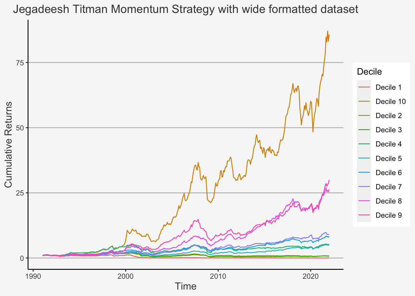
Finally, let’s calculate the summary statistics
df_mom <- as.data.frame(cbind(Dates, EW_Return_Mom_d1, EW_Return_Mom_d2, EW_Return_Mom_d3, EW_Return_Mom_d4,
                              EW_Return_Mom_d5, EW_Return_Mom_d6, EW_Return_Mom_d7, EW_Return_Mom_d8, EW_Return_Mom_d9, EW_Return_Mom_d10))

colnames(df_mom) <- c("Date", "Decile 1", "Decile 2", "Decile 3", "Decile 4", "Decile 5", "Decile 6", "Decile 7", "Decile 8", "Decile 9", "Decile 10")

# Transform into long format
df_mom_long <- df_mom %>%
  mutate(Date = as.Date(Date)) %>%
  gather(Decile, value, -c(Date))

colnames(df_mom_long) <- c("Date_t", "Decile", "EW_Ret_mean_t")

df_mom_long %>%
  subset(Decile != "NA") %>%
  group_by(Decile) %>%
  mutate(Annualised_Mean_Return = round((1+mean(EW_Ret_mean_t))^12 -1, 5),
         Annualised_SD = round(sd(EW_Ret_mean_t)*sqrt(12), 5),
         Sharpe_Ratio = round(Annualised_Mean_Return/Annualised_SD,5)) %>%
  select(Decile, Annualised_Mean_Return, Annualised_SD, Sharpe_Ratio) %>%
  unique()
## # A tibble: 10 × 4
## # Groups: Decile [10]
## Decile Annualised_Mean_Return Annualised_SD Sharpe_Ratio
## <chr> <dbl> <dbl> <dbl>
## 1 Decile 1 -0.0997 0.283 -0.352
## 2 Decile 2 0.0111 0.202 0.0549
## 3 Decile 3 0.0119 0.188 0.0635
## 4 Decile 4 0.0720 0.177 0.407
## 5 Decile 5 0.0670 0.158 0.423
## 6 Decile 6 0.0824 0.150 0.548
## 7 Decile 7 0.0850 0.146 0.581
## 8 Decile 8 0.124 0.150 0.824
## 9 Decile 9 0.129 0.156 0.828
## 10 Decile 10 0.172 0.179 0.9626.5.4.1.2 Long-format factor construction
# Let's run the experiment for the reduced data frame
tic_sub <- unique(names(read.csv("~/Desktop/Master UZH/Data/A4_dataset_04_Ex_Session.txt", header = T, sep = "\t")))
# Get 347 companies
CH_data_total_monthly <- read.csv("~/Desktop/CH_data_total_monthly.csv", header = T, sep = ",")
CH_data_total_monthly_clean <- CH_data_total_monthly[!duplicated(CH_data_total_monthly[c("Date_t", "Ticker")]),]

# Only get the respective columns
CH_data_total_mont <- CH_data_total_monthly_clean %>%
  subset(Ticker %in% tic_sub) %>%
  select(Date_t, Ticker, Adj_Close) %>%
  mutate(Date_t = as.Date(Date_t),
         Date_t = as.yearmon(Date_t))

# Control for extreme values
CH_data_total_monthly_sub <- CH_data_total_mont %>%
  arrange(Date_t) %>%
  select(Date_t, Ticker, Adj_Close) %>%
  group_by(Ticker) %>%
  mutate(Ret_Adj = (Adj_Close - lag(Adj_Close, 1))/lag(Adj_Close,1)) %>%
  na.omit() %>%
  ungroup() %>%
  group_by(Date_t) %>%
  mutate(Extreme_Values = quantile(Ret_Adj, p = 0.999),
         Extreme_Indicator = ifelse(Ret_Adj <= Extreme_Values, 1, NA),
         Ret_Adj = Ret_Adj * Extreme_Indicator) %>%
  ungroup()

# Get the lagged values to ensure that we have a HPR of 6 periods!
# Since we go 6 periods behind and take the cum ret from period -6 to period -1 to obtain the HPR from period -5 to 0.

# Idea: If we do it like this, we account for gaps in the data. E.g. if two observational periods were on Aug 1990 and then on Aug 1991, the gap would be 12 periods. Thus, this would not constitute a HPR of 6 periods, but 12. In order to ensure we only ever get HPR of 6 periods, we need to create the indicator which shows how many periods (in months) two dates are apart from one another. This must equal 6 and not more!

CH_data_total_monthly_sub_lag <- CH_data_total_monthly_sub %>%
  group_by(Ticker) %>%
  mutate(lag6 = round(12*(Date_t - lag(Date_t, n=5)))/5)

# Get the adjustred returns to form the PF on
CH_data_total_monthly_sub_cumret <- CH_data_total_monthly_sub_lag %>%
  group_by(Ticker) %>%
  mutate(Log_Ret_Adj = lag(log(1+Ret_Adj), n = 1),
         Sum_Ret = roll_sum(Log_Ret_Adj, 6),
         Cum_Ret = exp(Sum_Ret) - 1) %>%
  na.omit() %>%
  ungroup()

# Assign rankings
CH_data_total_monthly_sub_rank <- CH_data_total_monthly_sub_cumret %>%
  filter(.,  lag6 ==1) %>%
  group_by(Date_t) %>%
  # Here we form the groups (ranks)
  mutate(Decile = as.numeric(cut(Cum_Ret,
               breaks = quantile(Cum_Ret,
                                 probs = seq(0, 1, length = 11),
                                 na.rm = TRUE,
                                 type = 4),
               include.lowest = TRUE)),
         p1 = quantile(Cum_Ret, 0.1),
         p2 = quantile(Cum_Ret, 0.2),
         p3 = quantile(Cum_Ret, 0.3),
         p4 = quantile(Cum_Ret, 0.4),
         p5 = quantile(Cum_Ret, 0.5),
         p6 = quantile(Cum_Ret, 0.6),
         p7 = quantile(Cum_Ret, 0.7),
         p8 = quantile(Cum_Ret, 0.8),
         p9 = quantile(Cum_Ret, 0.9)) %>%
  ungroup()

# Select only certain columns
CH_data_total_monthly_sub_rank_2_lag <- CH_data_total_monthly_sub_rank %>%
  select(Date_t, Ticker, Decile)

# Merge two df
CH_data_total_monthly_sub_rank_tot <- CH_data_total_monthly_sub_lag %>% ungroup() %>%
    filter(., lag6 == 1 ) %>%
    left_join(CH_data_total_monthly_sub_rank_2_lag, by = c("Ticker"="Ticker", "Date_t" = "Date_t")) %>%
    select(Ticker,Date_t,Ret_Adj,Decile) %>%
    arrange(Ticker,Date_t) %>%
    group_by(Date_t,Decile) %>%
    mutate(momr = mean(Ret_Adj)) %>% ungroup() %>%
    select(Date_t,Decile,momr) %>% unique()

# Create mean returns
CH_data_EW_Ret <- CH_data_total_monthly_sub_rank_tot %>% group_by(Date_t, Decile) %>%
  mutate(EW_Ret_mean_t = mean(momr, na.rm = T),
         EW_Ret_sd_t = sd(momr, na.rm = T)) %>%
    select(Date_t,Decile,EW_Ret_mean_t,EW_Ret_sd_t) %>%
  ungroup() %>%
  unique() %>%
  arrange(Date_t,Decile)

CH_data_Cum_Ret <- CH_data_EW_Ret %>% group_by(Decile) %>%
  mutate(cum_ret = cumprod(1+EW_Ret_mean_t))

ewretdat2 <- CH_data_Cum_Ret %>% mutate(Decile = as.factor(Decile)) %>% mutate(Date_t = as.Date(Date_t)) %>% subset(!is.na(cum_ret) & !is.na(Decile))

ggplot(data = ewretdat2) +
    geom_line(mapping = aes(x =Date_t ,y = cum_ret ,color = Decile), size = 0.5 ) +
    ggtitle("Jegadeesh Titman Momentum Strategy with long formatted dataset") +
  ylab("Cumulative Returns") + xlab("Time") +
theme(plot.title= element_text(size=14, color="grey26",
hjust=0.5,
lineheight=1.2), panel.background = element_rect(fill="#f7f7f7"),
panel.grid.major.y = element_line(size = 0.5, linetype = "solid", color = "grey"),
panel.grid.minor = element_blank(),
panel.grid.major.x = element_blank(),
plot.background = element_rect(fill="#f7f7f7", color = "#f7f7f7"), axis.title.x = element_text(color="grey26", size=12),
axis.title.y = element_text(color="grey26", size=12),
axis.line = element_line(color = "black")) 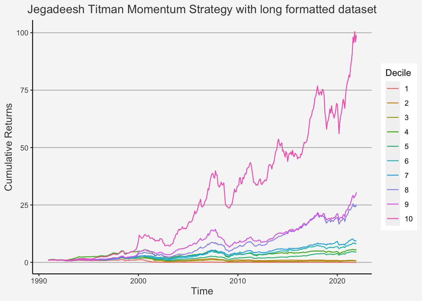
Finally, let’s calculate the summary statistics
CH_data_EW_Ret %>%
  subset(Decile != "NA") %>%
  group_by(Decile) %>%
  mutate(Annualised_Mean_Return = round((1+mean(EW_Ret_mean_t))^12 -1,5),
         Annualised_SD = round(sd(EW_Ret_mean_t)*sqrt(12), 5),
         Sharpe_Ratio = round(Annualised_Mean_Return/Annualised_SD,5)) %>%
  select(Decile, Annualised_Mean_Return, Annualised_SD, Sharpe_Ratio) %>%
  unique()
## # A tibble: 10 × 4
## # Groups: Decile [10]
## Decile Annualised_Mean_Return Annualised_SD Sharpe_Ratio
## <dbl> <dbl> <dbl> <dbl>
## 1 1 -0.103 0.287 -0.359
## 2 2 0.0137 0.199 0.0685
## 3 3 0.00573 0.189 0.0304
## 4 4 0.0742 0.178 0.416
## 5 5 0.0638 0.157 0.406
## 6 6 0.0826 0.149 0.553
## 7 7 0.0858 0.143 0.600
## 8 8 0.122 0.149 0.817
## 9 9 0.129 0.153 0.843
## 10 10 0.177 0.177 0.9996.5.4.2 The Size Factor
This is the long-format construction of the size factor based on the data downloaded.
# Let's run the experiment for the reduced data frame
tic_sub <- unique(names(read.csv("~/Desktop/Master UZH/Data/A4_dataset_04_Ex_Session.txt", header = T, sep = "\t")))
# Get 347 companies
CH_data_total_monthly <- read.csv("~/Desktop/CH_data_total_monthly.csv", header = T, sep = ",")
CH_data_total_monthly_clean <- CH_data_total_monthly[!duplicated(CH_data_total_monthly[c("Date_t", "Ticker")]),]

# Only get the respective columns
CH_data_total_mont <- CH_data_total_monthly_clean %>%
  subset(Ticker %in% tic_sub) %>%
  select(Date_t, Ticker, Adj_Close, Close, Num_Shares)

# Control for extreme values
CH_data_total_monthly_sub_Size <- CH_data_total_mont %>%
  arrange(Date_t)  %>%
  group_by(Ticker) %>%
  mutate(Ret_Adj = (Adj_Close - lag(Adj_Close, 1))/lag(Adj_Close,1)) %>%
  na.omit() %>%
  ungroup() %>%
  group_by(Date_t) %>%
  mutate(Extreme_Values = quantile(Ret_Adj, p = 0.999),
         Extreme_Indicator = ifelse(Ret_Adj <= Extreme_Values, 1, NA),
         Ret_Adj = Ret_Adj * Extreme_Indicator) %>%
  ungroup()

CH_data_total_monthly_sub_cumret_Size <- CH_data_total_monthly_sub_Size %>%
  group_by(Ticker) %>%
  mutate(Shares_Out_lagged = lag(Num_Shares, n = 1),
         Price_close_lagged = lag(Close, n = 1),
         Market_Cap = Shares_Out_lagged * Price_close_lagged) %>%
  na.omit() %>%
  ungroup()

# Assign rankings
CH_data_total_monthly_sub_rank_Size <- CH_data_total_monthly_sub_cumret_Size %>%
  group_by(Date_t) %>%
  # Here we form the groups (ranks)
  mutate(Decile = as.numeric(cut(Market_Cap,
               breaks = quantile(Market_Cap,
                                 probs = seq(0, 1, length = 11),
                                 na.rm = TRUE,
                                 type = 4),
               include.lowest = TRUE)),
         p1 = quantile(Market_Cap, 0.1),
         p2 = quantile(Market_Cap, 0.2),
         p3 = quantile(Market_Cap, 0.3),
         p4 = quantile(Market_Cap, 0.4),
         p5 = quantile(Market_Cap, 0.5),
         p6 = quantile(Market_Cap, 0.6),
         p7 = quantile(Market_Cap, 0.7),
         p8 = quantile(Market_Cap, 0.8),
         p9 = quantile(Market_Cap, 0.9)) %>%
  ungroup()

# Create mean returns
CH_data_EW_Ret_Size <- CH_data_total_monthly_sub_rank_Size %>% group_by(Date_t, Decile) %>%
  mutate(EW_Ret_mean_t = mean(Ret_Adj, na.rm = T),
         EW_Ret_sd_t = sd(Ret_Adj, na.rm = T)) %>%
    select(Date_t,Decile,EW_Ret_mean_t,EW_Ret_sd_t) %>%
  ungroup() %>%
  unique() %>%
  arrange(Date_t,Decile)

CH_data_Cum_Ret_Size <- CH_data_EW_Ret_Size %>% group_by(Decile) %>%
  mutate(cum_ret = cumprod(1+EW_Ret_mean_t))

EW_Size <- CH_data_Cum_Ret_Size %>% mutate(Decile = as.factor(Decile)) %>% mutate(Date_t = as.Date(Date_t))

ggplot(data = EW_Size) +
    geom_line(mapping = aes(x =Date_t ,y = cum_ret ,color = Decile), size = 0.5 ) +
    ggtitle("Size Strategy with long formatted dataset") +
  ylab("Cumulative Returns") + xlab("Time") +
theme(plot.title= element_text(size=14, color="grey26",
hjust=0.5,
lineheight=1.2), panel.background = element_rect(fill="#f7f7f7"),
panel.grid.major.y = element_line(size = 0.5, linetype = "solid", color = "grey"),
panel.grid.minor = element_blank(),
panel.grid.major.x = element_blank(),
plot.background = element_rect(fill="#f7f7f7", color = "#f7f7f7"), axis.title.x = element_text(color="grey26", size=12),
axis.title.y = element_text(color="grey26", size=12),
axis.line = element_line(color = "black")) 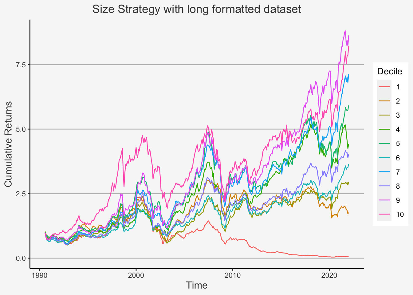
Finally, let’s calculate the summary statistics
CH_data_EW_Ret_Size %>%
  group_by(Decile) %>%
  mutate(Annualised_Mean_Return = (1+mean(EW_Ret_mean_t))^12 -1,
         Annualised_SD = sd(EW_Ret_mean_t)*sqrt(12),
         Sharpe_Ratio = Annualised_Mean_Return/Annualised_SD) %>%
  select(Decile, Annualised_Mean_Return, Annualised_SD, Sharpe_Ratio) %>%
  unique()
## # A tibble: 10 × 4
## # Groups: Decile [10]
## Decile Annualised_Mean_Return Annualised_SD Sharpe_Ratio
## <dbl> <dbl> <dbl> <dbl>
## 1 1 -0.0679 0.210 -0.324
## 2 2 0.0332 0.171 0.194
## 3 3 0.0488 0.162 0.302
## 4 4 0.0627 0.165 0.381
## 5 5 0.0750 0.177 0.423
## 6 6 0.0555 0.161 0.346
## 7 7 0.0780 0.160 0.489
## 8 8 0.0609 0.171 0.356
## 9 9 0.0889 0.180 0.492
## 10 10 0.0857 0.174 0.4926.5.4.3 The Value Factor
This is the long-format construction of the value factor based on the data downloaded.
# Let's run the experiment for the reduced data frame
tic_sub <- unique(names(read.csv("~/Desktop/Master UZH/Data/A4_dataset_04_Ex_Session.txt", header = T, sep = "\t")))
# Get 347 companies
CH_data_total_monthly <- read.csv("~/Desktop/CH_data_total_monthly.csv", header = T, sep = ",")
CH_data_total_monthly_clean <- CH_data_total_monthly[!duplicated(CH_data_total_monthly[c("Date_t", "Ticker")]),]

# Only get the respective columns
CH_data_total_mont <- CH_data_total_monthly_clean %>%
  subset(Ticker %in% tic_sub) %>%
  select(Date_t, Ticker, Adj_Close, Close, Num_Shares, Total_Assets_t, Total_Liab_t, Total_Eq_t)

# Control for extreme values
CH_data_total_monthly_sub_Value <- CH_data_total_mont %>%
  arrange(Date_t)  %>%
  group_by(Ticker) %>%
  mutate(Ret_Adj = (Adj_Close - lag(Adj_Close, 1))/lag(Adj_Close,1)) %>%
  na.omit() %>%
  ungroup() %>%
  group_by(Date_t) %>%
  mutate(Extreme_Values = quantile(Ret_Adj, p = 0.999),
         Extreme_Indicator = ifelse(Ret_Adj <= Extreme_Values, 1, NA),
         Ret_Adj = Ret_Adj * Extreme_Indicator) %>%
  ungroup()

CH_data_total_monthly_sub_cumret_Value <- CH_data_total_monthly_sub_Value %>%
  group_by(Ticker) %>%
  mutate(Shares_Out_lagged = lag(Num_Shares, n = 1),
         Price_close_lagged = lag(Close, n = 1),
         Market_Cap = Shares_Out_lagged * Price_close_lagged,
         Total_Eq_t = Total_Assets_t - Total_Liab_t,
         B2M = lag(Total_Eq_t, n = 7) /Market_Cap) %>%
  na.omit() %>%
  ungroup()

# Assign rankings
CH_data_total_monthly_sub_rank_Value <- CH_data_total_monthly_sub_cumret_Value %>%
  group_by(Date_t) %>%
  # Here we form the groups (ranks)
  mutate(Decile = as.numeric(cut(B2M,
               breaks = quantile(B2M,
                                 probs = seq(0, 1, length = 11),
                                 na.rm = TRUE,
                                 type = 4),
               include.lowest = TRUE)),
         p1 = quantile(B2M, 0.1),
         p2 = quantile(B2M, 0.2),
         p3 = quantile(B2M, 0.3),
         p4 = quantile(B2M, 0.4),
         p5 = quantile(B2M, 0.5),
         p6 = quantile(B2M, 0.6),
         p7 = quantile(B2M, 0.7),
         p8 = quantile(B2M, 0.8),
         p9 = quantile(B2M, 0.9)) %>%
  ungroup()

# Create mean returns
CH_data_EW_Ret_Value <- CH_data_total_monthly_sub_rank_Value %>% group_by(Date_t, Decile) %>%
  mutate(EW_Ret_mean_t = mean(Ret_Adj, na.rm = T),
         EW_Ret_sd_t = sd(Ret_Adj, na.rm = T)) %>%
    select(Date_t,Decile,EW_Ret_mean_t,EW_Ret_sd_t) %>%
  ungroup() %>%
  unique() %>%
  arrange(Date_t,Decile)

CH_data_Cum_Ret_Value <- CH_data_EW_Ret_Value %>% group_by(Decile) %>%
  mutate(cum_ret = cumprod(1+EW_Ret_mean_t))

EW_Value <- CH_data_Cum_Ret_Value %>% mutate(Decile = as.factor(Decile)) %>% mutate(Date_t = as.Date(Date_t))

ggplot(data = EW_Value) +
    geom_line(mapping = aes(x =Date_t ,y = cum_ret ,color = Decile), size = 0.5 ) +
    ggtitle("Value Strategy with long formatted dataset") +
  ylab("Cumulative Returns") + xlab("Time") +
theme(plot.title= element_text(size=14, color="grey26",
hjust=0.5,
lineheight=1.2), panel.background = element_rect(fill="#f7f7f7"),
panel.grid.major.y = element_line(size = 0.5, linetype = "solid", color = "grey"),
panel.grid.minor = element_blank(),
panel.grid.major.x = element_blank(),
plot.background = element_rect(fill="#f7f7f7", color = "#f7f7f7"), axis.title.x = element_text(color="grey26", size=12),
axis.title.y = element_text(color="grey26", size=12),
axis.line = element_line(color = "black")) 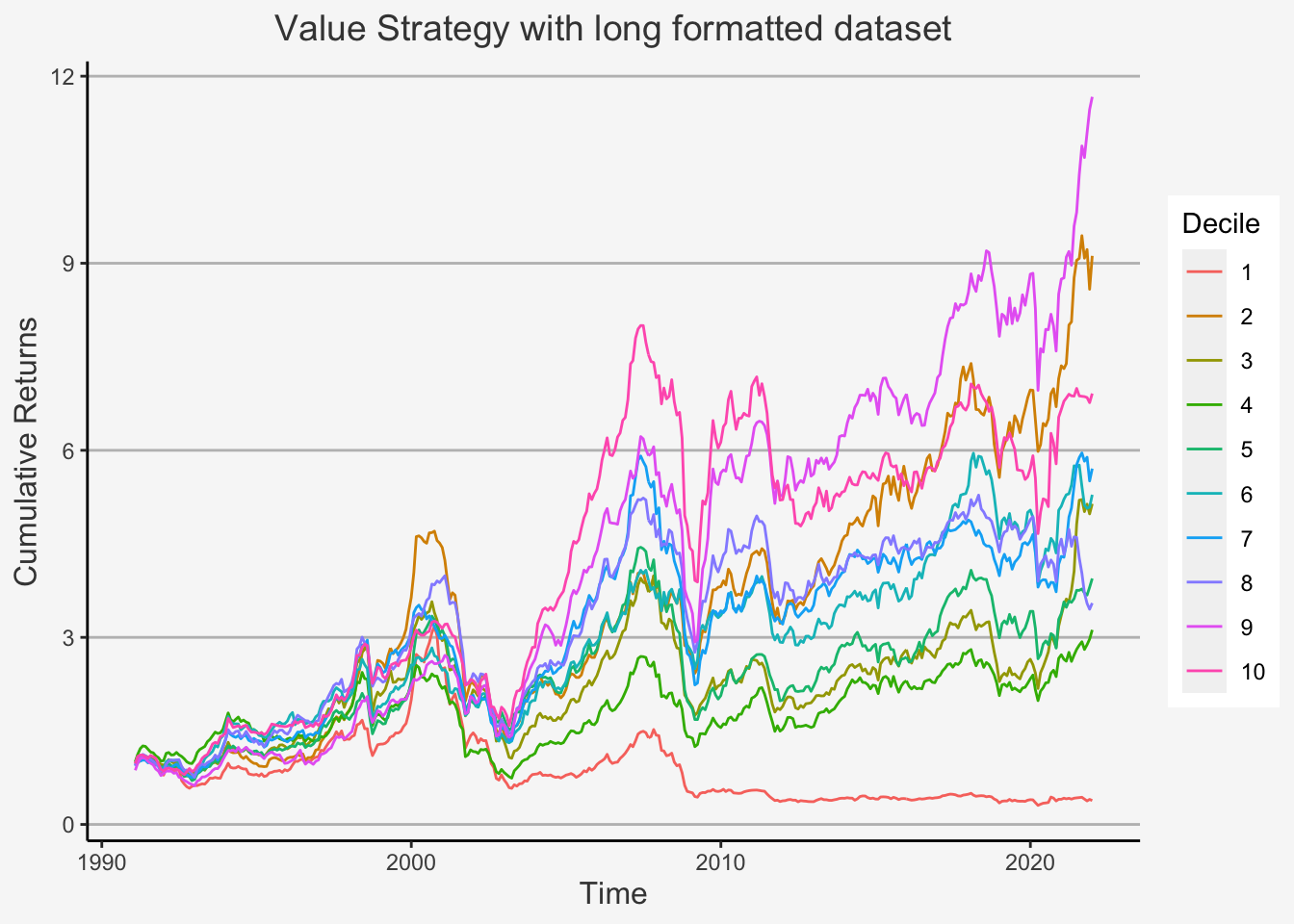
Finally, let’s calculate the summary statistics
CH_data_EW_Ret_Value %>%
  group_by(Decile) %>%
  mutate(Annualised_Mean_Return = (1+mean(EW_Ret_mean_t))^12 -1,
         Annualised_SD = sd(EW_Ret_mean_t)*sqrt(12),
         Sharpe_Ratio = Annualised_Mean_Return/Annualised_SD) %>%
  select(Decile, Annualised_Mean_Return, Annualised_SD, Sharpe_Ratio) %>%
  unique()
## # A tibble: 10 × 4
## # Groups: Decile [10]
## Decile Annualised_Mean_Return Annualised_SD Sharpe_Ratio
## <dbl> <dbl> <dbl> <dbl>
## 1 1 -0.00841 0.209 -0.0403
## 2 2 0.0903 0.173 0.521
## 3 3 0.0730 0.186 0.392
## 4 4 0.0535 0.173 0.309
## 5 5 0.0602 0.168 0.358
## 6 6 0.0697 0.166 0.421
## 7 7 0.0715 0.161 0.445
## 8 8 0.0558 0.164 0.340
## 9 9 0.0984 0.171 0.574
## 10 10 0.0782 0.162 0.4836.5.4.4 The Profitability Factor
This is the long-format construction of the profitability factor based on the data downloaded.
# Let's run the experiment for the reduced data frame
tic_sub <- unique(names(read.csv("~/Desktop/Master UZH/Data/A4_dataset_04_Ex_Session.txt", header = T, sep = "\t")))
# Get 347 companies
CH_data_total_monthly <- read.csv("~/Desktop/CH_data_total_monthly.csv", header = T, sep = ",")
CH_data_total_monthly_clean <- CH_data_total_monthly[!duplicated(CH_data_total_monthly[c("Date_t", "Ticker")]),]

# Only get the respective columns
CH_data_total_mont <- CH_data_total_monthly_clean %>%
  subset(Ticker %in% tic_sub) %>%
  select(Date_t, Ticker, Adj_Close, Gross_Inc_t, Operating_Exp_t, Interest_Exp_t, Total_Eq_t)

# Control for extreme values
CH_data_total_monthly_sub_Profit <- CH_data_total_mont %>%
  arrange(Date_t)  %>%
  group_by(Ticker) %>%
  mutate(Ret_Adj = (Adj_Close - lag(Adj_Close, 1))/lag(Adj_Close,1)) %>%
  na.omit() %>%
  ungroup() %>%
  group_by(Date_t) %>%
  mutate(Extreme_Values = quantile(Ret_Adj, p = 0.999),
         Extreme_Indicator = ifelse(Ret_Adj <= Extreme_Values, 1, NA),
         Ret_Adj = Ret_Adj * Extreme_Indicator) %>%
  ungroup()

CH_data_total_monthly_sub_cumret_Profit <- CH_data_total_monthly_sub_Profit %>%
  group_by(Ticker) %>%
  mutate(Profit_lead = (Gross_Inc_t - Operating_Exp_t - Interest_Exp_t)/Total_Eq_t,
         Profit = lag(Profit_lead, n = 1)) %>%
  na.omit() %>%
  ungroup()

# Assign rankings
CH_data_total_monthly_sub_rank_Profit <- CH_data_total_monthly_sub_cumret_Profit %>%
  group_by(Date_t) %>%
  # Here we form the groups (ranks)
  mutate(Decile = as.numeric(cut(Profit,
               breaks = quantile(Profit,
                                 probs = seq(0, 1, length = 11),
                                 na.rm = TRUE,
                                 type = 4),
               include.lowest = TRUE)),
         p1 = quantile(Profit, 0.1),
         p2 = quantile(Profit, 0.2),
         p3 = quantile(Profit, 0.3),
         p4 = quantile(Profit, 0.4),
         p5 = quantile(Profit, 0.5),
         p6 = quantile(Profit, 0.6),
         p7 = quantile(Profit, 0.7),
         p8 = quantile(Profit, 0.8),
         p9 = quantile(Profit, 0.9)) %>%
  ungroup()

# Create mean returns
CH_data_EW_Ret_Profit <- CH_data_total_monthly_sub_rank_Profit %>% group_by(Date_t, Decile) %>%
  mutate(EW_Ret_mean_t = mean(Ret_Adj, na.rm = T),
         EW_Ret_sd_t = sd(Ret_Adj, na.rm = T)) %>%
    select(Date_t,Decile,EW_Ret_mean_t,EW_Ret_sd_t) %>%
  ungroup() %>%
  unique() %>%
  arrange(Date_t,Decile)

CH_data_Cum_Ret_Profit <- CH_data_EW_Ret_Profit %>% group_by(Decile) %>%
  mutate(cum_ret = cumprod(1+EW_Ret_mean_t))

EW_Profit <- CH_data_Cum_Ret_Profit %>% mutate(Decile = as.factor(Decile)) %>% mutate(Date_t = as.Date(Date_t))

ggplot(data = EW_Profit) +
    geom_line(mapping = aes(x =Date_t ,y = cum_ret ,color = Decile), size = 0.5 ) +
    ggtitle("Operating Profitability Strategy with long formatted dataset") +
  ylab("Cumulative Returns") + xlab("Time") +
theme(plot.title= element_text(size=14, color="grey26",
hjust=0.5,
lineheight=1.2), panel.background = element_rect(fill="#f7f7f7"),
panel.grid.major.y = element_line(size = 0.5, linetype = "solid", color = "grey"),
panel.grid.minor = element_blank(),
panel.grid.major.x = element_blank(),
plot.background = element_rect(fill="#f7f7f7", color = "#f7f7f7"), axis.title.x = element_text(color="grey26", size=12),
axis.title.y = element_text(color="grey26", size=12),
axis.line = element_line(color = "black")) 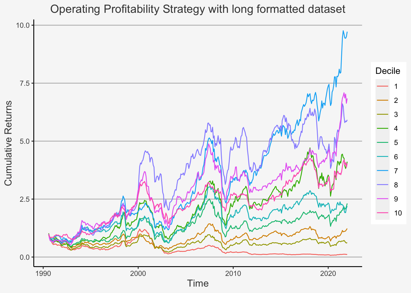
Finally, let’s calculate the summary statistics
CH_data_EW_Ret_Profit %>%
  group_by(Decile) %>%
  mutate(Annualised_Mean_Return = (1+mean(EW_Ret_mean_t))^12 -1,
         Annualised_SD = sd(EW_Ret_mean_t)*sqrt(12),
         Sharpe_Ratio = Annualised_Mean_Return/Annualised_SD) %>%
  select(Decile, Annualised_Mean_Return, Annualised_SD, Sharpe_Ratio) %>%
  unique()
## # A tibble: 10 × 4
## # Groups: Decile [10]
## Decile Annualised_Mean_Return Annualised_SD Sharpe_Ratio
## <dbl> <dbl> <dbl> <dbl>
## 1 1 -0.0411 0.227 -0.181
## 2 2 0.0256 0.191 0.134
## 3 3 0.0100 0.221 0.0455
## 4 4 0.0676 0.201 0.336
## 5 5 0.0469 0.194 0.241
## 6 6 0.0434 0.186 0.234
## 7 7 0.0893 0.163 0.547
## 8 8 0.0763 0.186 0.411
## 9 9 0.0793 0.175 0.453
## 10 10 0.0565 0.147 0.3866.5.4.5 The Investment Factor
This is the long-format construction of the investment factor based on the data downloaded.
# Let's run the experiment for the reduced data frame
tic_sub <- unique(names(read.csv("~/Desktop/Master UZH/Data/A4_dataset_04_Ex_Session.txt", header = T, sep = "\t")))
# Get 347 companies
CH_data_total_monthly <- read.csv("~/Desktop/CH_data_total_monthly.csv", header = T, sep = ",")
CH_data_total_monthly_clean <- CH_data_total_monthly[!duplicated(CH_data_total_monthly[c("Date_t", "Ticker")]),]

# Only get the respective columns
CH_data_total_mont <- CH_data_total_monthly_clean %>%
  subset(Ticker %in% tic_sub) %>%
  select(Date_t, Ticker, Adj_Close, Total_Assets_t)

# Control for extreme values
CH_data_total_monthly_sub_Invest <- CH_data_total_mont %>%
  arrange(Date_t)  %>%
  group_by(Ticker) %>%
  mutate(Ret_Adj = (Adj_Close - lag(Adj_Close, 1))/lag(Adj_Close,1)) %>%
  na.omit() %>%
  ungroup() %>%
  group_by(Date_t) %>%
  mutate(Extreme_Values = quantile(Ret_Adj, p = 0.999),
         Extreme_Indicator = ifelse(Ret_Adj <= Extreme_Values, 1, NA),
         Ret_Adj = Ret_Adj * Extreme_Indicator) %>%
  ungroup()

CH_data_total_monthly_sub_cumret_Invest <- CH_data_total_monthly_sub_Invest %>%
  group_by(Ticker) %>%
  mutate(Invest_lead = (Total_Assets_t - lag(Total_Assets_t, n = 12))/lag(Total_Assets_t, n = 12),
         Invest = lag(Invest_lead, n = 1)) %>%
  na.omit() %>%
  ungroup()

# Assign rankings
CH_data_total_monthly_sub_rank_Invest <- CH_data_total_monthly_sub_cumret_Invest %>%
  group_by(Date_t) %>%
  # Here we form the groups (ranks)
  mutate(Decile = as.numeric(cut(Invest,
               breaks = quantile(Invest,
                                 probs = seq(0, 1, length = 11),
                                 na.rm = TRUE,
                                 type = 4),
               include.lowest = TRUE)),
         p1 = quantile(Invest, 0.1),
         p2 = quantile(Invest, 0.2),
         p3 = quantile(Invest, 0.3),
         p4 = quantile(Invest, 0.4),
         p5 = quantile(Invest, 0.5),
         p6 = quantile(Invest, 0.6),
         p7 = quantile(Invest, 0.7),
         p8 = quantile(Invest, 0.8),
         p9 = quantile(Invest, 0.9)) %>%
  ungroup()

# Create mean returns
CH_data_EW_Ret_Invest <- CH_data_total_monthly_sub_rank_Invest %>% group_by(Date_t, Decile) %>%
  mutate(EW_Ret_mean_t = mean(Ret_Adj, na.rm = T),
         EW_Ret_sd_t = sd(Ret_Adj, na.rm = T)) %>%
    select(Date_t,Decile,EW_Ret_mean_t,EW_Ret_sd_t) %>%
  ungroup() %>%
  unique() %>%
  arrange(Date_t,Decile)

CH_data_Cum_Ret_Invest <- CH_data_EW_Ret_Invest %>% group_by(Decile) %>%
  mutate(cum_ret = cumprod(1+EW_Ret_mean_t))

EW_Invest <- CH_data_Cum_Ret_Invest %>% mutate(Decile = as.factor(Decile)) %>% mutate(Date_t = as.Date(Date_t))

ggplot(data = EW_Invest) +
    geom_line(mapping = aes(x =Date_t ,y = cum_ret ,color = Decile), size = 0.5 ) +
    ggtitle("Investment Growth Strategy with long formatted dataset") +
  ylab("Cumulative Returns") + xlab("Time") +
theme(plot.title= element_text(size=14, color="grey26",
hjust=0.5,
lineheight=1.2), panel.background = element_rect(fill="#f7f7f7"),
panel.grid.major.y = element_line(size = 0.5, linetype = "solid", color = "grey"),
panel.grid.minor = element_blank(),
panel.grid.major.x = element_blank(),
plot.background = element_rect(fill="#f7f7f7", color = "#f7f7f7"), axis.title.x = element_text(color="grey26", size=12),
axis.title.y = element_text(color="grey26", size=12),
axis.line = element_line(color = "black")) 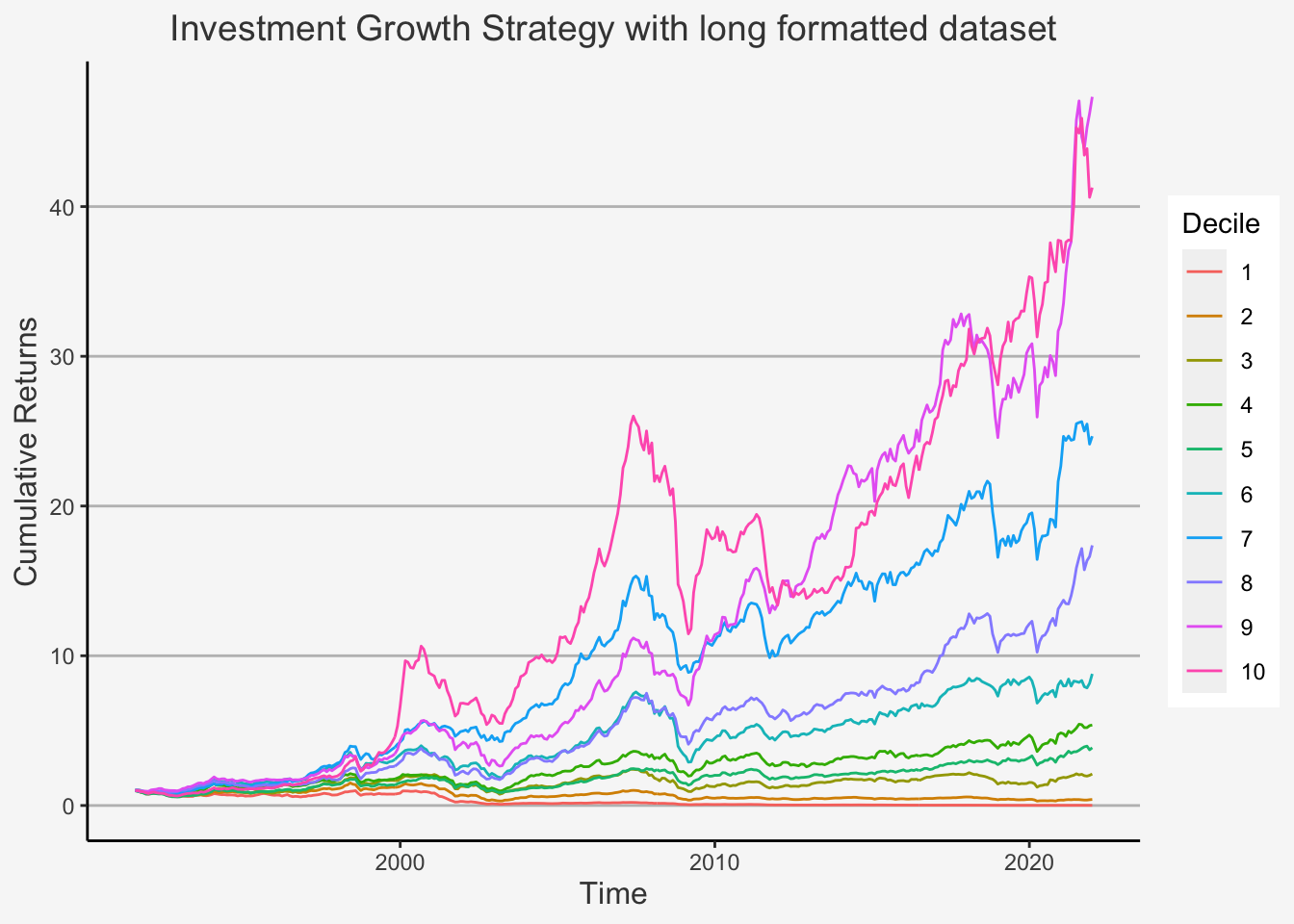
Finally, let’s calculate the summary statistics
CH_data_EW_Ret_Invest %>%
  group_by(Decile) %>%
  mutate(Annualised_Mean_Return = (1+mean(EW_Ret_mean_t))^12 -1,
         Annualised_SD = sd(EW_Ret_mean_t)*sqrt(12),
         Sharpe_Ratio = Annualised_Mean_Return/Annualised_SD) %>%
  select(Decile, Annualised_Mean_Return, Annualised_SD, Sharpe_Ratio) %>%
  unique()
## # A tibble: 10 × 4
## # Groups: Decile [10]
## Decile Annualised_Mean_Return Annualised_SD Sharpe_Ratio
## <dbl> <dbl> <dbl> <dbl>
## 1 1 -0.115 0.233 -0.494
## 2 2 -0.0110 0.191 -0.0576
## 3 3 0.0423 0.184 0.230
## 4 4 0.0699 0.157 0.445
## 5 5 0.0578 0.153 0.377
## 6 6 0.0885 0.164 0.539
## 7 7 0.122 0.145 0.842
## 8 8 0.112 0.159 0.705
## 9 9 0.150 0.164 0.913
## 10 10 0.148 0.183 0.8096.5.4.6 The Betting against Beta Factor
# Let's run the experiment for the reduced data frame
tic_sub <- unique(names(read.csv("~/Desktop/Master UZH/Data/A4_dataset_04_Ex_Session.txt", header = T, sep = "\t")))
# Get 347 companies
CH_data_total_monthly <- read.csv("~/Desktop/CH_data_total_monthly.csv", header = T, sep = ",")
CH_data_total_monthly_clean <- CH_data_total_monthly[!duplicated(CH_data_total_monthly[c("Date_t", "Ticker")]),]

# Only get the respective columns
CH_data_total_mont <- CH_data_total_monthly_clean %>%
  subset(Ticker %in% tic_sub) %>%
  select(Date_t, Ticker, Adj_Close, Total_Assets_t)

# Control for extreme values
CH_data_total_monthly_sub_BAB <- CH_data_total_mont %>%
  arrange(Date_t)  %>%
  group_by(Ticker) %>%
  mutate(Ret_Adj = (Adj_Close - lag(Adj_Close, 1))/lag(Adj_Close,1)) %>%
  na.omit() %>%
  ungroup() %>%
  group_by(Date_t) %>%
  mutate(Extreme_Values = quantile(Ret_Adj, p = 1),
         Extreme_Indicator = ifelse(Ret_Adj <= Extreme_Values, 1, NA),
         Ret_Adj = Ret_Adj * Extreme_Indicator) %>%
  ungroup()


# Let's also get the data on the Swiss Market Index as well as the risk free rate
rf <- read.csv("~/Desktop/Master UZH/Data/A2_dataset_02_Ex_Session.txt", header = T, sep = "\t")
rf_ts <- rf %>%
  subset((Date >= '1989-12-01') & (Date <= '2019-12-31')) %>%
  mutate(rf_annual = SWISS.CONFEDERATION.BOND.1.YEAR...RED..YIELD / 1000,
         rf_monthly =  (1 + rf_annual)^(1/12) - 1) %>%
  select(Date, rf_monthly)


SMI <-  read.csv("~/Desktop/Master UZH/Data/A2_dataset_03_Ex_Session.txt", header = T, sep = "\t")
SMI_ts <- SMI %>%
  subset((Date >= '1989-12-01') & (Date <= '2019-12-31')) %>%
  mutate(SMI_ret = (SMI - lag(SMI, 1))/lag(SMI, 1),
         rf_monthly = rf_ts$rf_monthly,
         SMI_rf_excess_ret = SMI_ret - rf_monthly)

# Now, let's calculate the excess returns
SMI_rf_ts_ret <- SMI_ts_ret - rf_ts_monthly
CH_data_total_monthly_sub_excess_ret_BAB <- left_join(SMI_ts, CH_data_total_monthly_sub_BAB, by = c("Date" = "Date_t")) %>%
  mutate(Excess_Ret_Adj = Ret_Adj - rf_monthly)

# Based on this, we can now have rolling regressions of the correlation as well as the standard deviations.
CH_data_total_monthly_weighted_BAB <- CH_data_total_monthly_sub_excess_ret_BAB %>%
  group_by(Ticker) %>%
  mutate(sd_roll_1_year = roll_sd(Excess_Ret_Adj, width = 12),
         corr_roll_5_year = roll_cor(Excess_Ret_Adj, SMI_rf_excess_ret, width = 60),
         sd_roll_1_year_Market = roll_sd(SMI_rf_excess_ret, width = 12),
         Beta_Est_raw = sd_roll_1_year/sd_roll_1_year_Market*corr_roll_5_year,
         Beta_Est_Adj = Beta_Est_raw*0.4 + 0.6*1) %>%
  ungroup() %>%
  subset(!is.na(Beta_Est_Adj)) %>%
  group_by(Date) %>%
  mutate(ranks_beta = rank(Beta_Est_Adj),
         mean_rank_beta = mean(ranks_beta, na.rm = T),
         portfolio_indicator_BAB =ifelse(ranks_beta > mean_rank_beta, 1, 0)) %>%
  ungroup() %>%
  group_by(Date, portfolio_indicator_BAB) %>%
  mutate(abs_dev = abs(ranks_beta - mean_rank_beta),
         sum_abs_dev = sum(abs_dev, na.rm = T),
         k = 2 / sum_abs_dev,
         weights_BAB = k*(ranks_beta - mean_rank_beta),
         Beta_Est_Weight_Adj = Beta_Est_Adj * weights_BAB) %>%
  ungroup()

# Assign rankings
CH_data_total_monthly_rank_BAB <- CH_data_total_monthly_weighted_BAB %>%
  group_by(Date) %>%
  mutate(Min_PF = n()) %>%
  subset(Min_PF >= 10) %>%
  mutate(Decile = as.numeric(cut(Beta_Est_Weight_Adj,
               breaks = quantile(Beta_Est_Weight_Adj,
                                 probs = seq(0, 1, length = 10),
                                 na.rm = TRUE,
                                 type = 4),
               include.lowest = TRUE)),
         p1 = quantile(Beta_Est_Weight_Adj, 0.1),
         p2 = quantile(Beta_Est_Weight_Adj, 0.2),
         p3 = quantile(Beta_Est_Weight_Adj, 0.3),
         p4 = quantile(Beta_Est_Weight_Adj, 0.4),
         p5 = quantile(Beta_Est_Weight_Adj, 0.5),
         p6 = quantile(Beta_Est_Weight_Adj, 0.6),
         p7 = quantile(Beta_Est_Weight_Adj, 0.7),
         p8 = quantile(Beta_Est_Weight_Adj, 0.8),
         p9 = quantile(Beta_Est_Weight_Adj, 0.9)) %>%
  ungroup()

# Create mean returns Decile
CH_data_EW_Ret_BAB <- CH_data_total_monthly_rank_BAB %>%
  group_by(Date, Decile) %>%
  mutate(EW_Ret_mean_t = 1/sum(Beta_Est_Weight_Adj)*sum(weights_BAB*Excess_Ret_Adj)) %>%
  select(Date, Decile, EW_Ret_mean_t) %>%
  ungroup() %>%
  unique() %>%
  arrange(Date, Decile)

# Create the cumulative returns
CH_data_Cum_Ret_BAB <- CH_data_EW_Ret_BAB %>%
  group_by(Decile) %>%
  mutate(cum_ret = cumprod(1+EW_Ret_mean_t))

EW_BAB <- CH_data_Cum_Ret_BAB %>%
  mutate(Decile = as.factor(Decile)) %>% mutate(Date = as.Date(Date))

EW_BAB %>%
  subset(Decile != 5) %>%
ggplot() +
    geom_line(mapping = aes(x =Date ,y = cum_ret ,color = Decile), size = 0.5) +
    ggtitle("BAB Strategy with long formatted dataset") +
  ylab("Cumulative Returns") + xlab("Time") +
theme(plot.title= element_text(size=14, color="grey26",
hjust=0.5,
lineheight=1.2), panel.background = element_rect(fill="#f7f7f7"),
panel.grid.major.y = element_line(size = 0.5, linetype = "solid", color = "grey"),
panel.grid.minor = element_blank(),
panel.grid.major.x = element_blank(),
plot.background = element_rect(fill="#f7f7f7", color = "#f7f7f7"), axis.title.x = element_text(color="grey26", size=12),
axis.title.y = element_text(color="grey26", size=12),
axis.line = element_line(color = "black")) 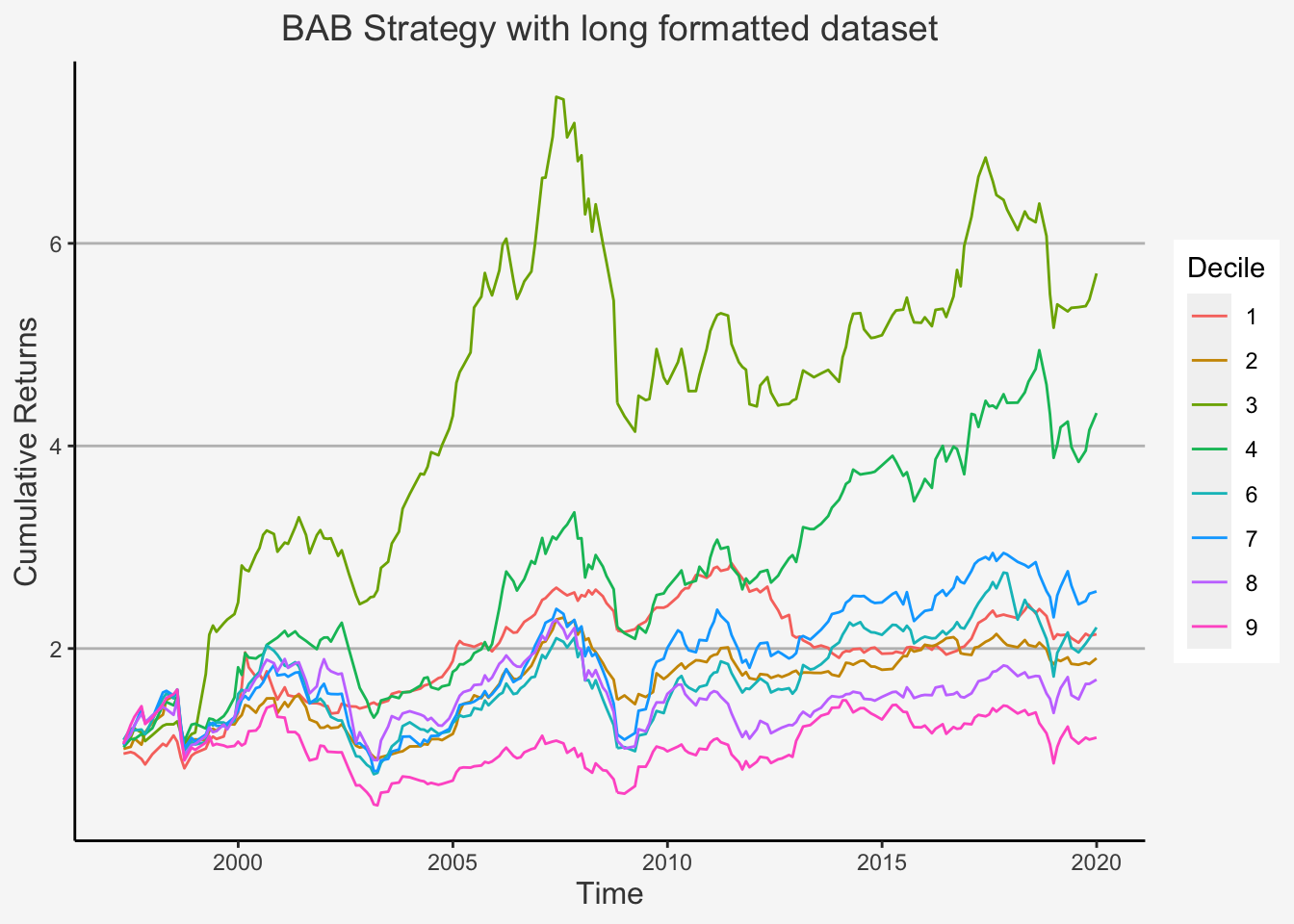
Finally, let’s calculate the summary statistics
CH_data_EW_Ret_BAB %>%
  group_by(Decile) %>%
  mutate(Annualised_Mean_Return = (1+mean(EW_Ret_mean_t))^12 -1,
         Annualised_SD = sd(EW_Ret_mean_t)*sqrt(12),
         Sharpe_Ratio = Annualised_Mean_Return/Annualised_SD) %>%
  select(Decile, Annualised_Mean_Return, Annualised_SD, Sharpe_Ratio) %>%
  unique()
## # A tibble: 9 × 4
## # Groups: Decile [9]
## Decile Annualised_Mean_Return Annualised_SD Sharpe_Ratio
## <dbl> <dbl> <dbl> <dbl>
## 1 1 0.0595 0.147 0.405
## 2 2 0.0522 0.147 0.356
## 3 3 0.134 0.199 0.674
## 4 4 0.114 0.185 0.616
## 5 5 -0.234 3.46 -0.0676
## 6 6 0.0773 0.224 0.346
## 7 7 0.0857 0.216 0.397
## 8 8 0.0611 0.227 0.269
## 9 9 0.0435 0.266 0.1636.5.5 Double-sorted Portfolios
We now have created the portfolio sorts for each of the factors under consideration and plotted the cumulative returns of each decile throughout time. Let’s now get one step further and calculate double-sorted portfolios based on the company size as well as the respective factor characteristic under consideration. Throughout, we will follow the approach of Fama and French (1993, 2015). That is, we will use the formulas specifically highlighted and used by both researchers during the construction for the US market and replicate their strategy for the Swiss market. The repsective factors can be found on Kenneth French’s webpage.
6.5.5.1 Small Minus Big
For the SMB factor, we will use an aggregate of double-sorted portfolios based on size as well as Value, Profitability and Investment, respectively. That is, we will double-sort the stocks based on size and each of the three distinct accounting measures and then create a long-short strategy for each double sort. Lastly, we will aggregate the three risk factors by creating an equal-weighted SMB factor consisting of all three sub-factors.
# Let's run the experiment for the reduced data frame
tic_sub <- unique(names(read.csv("~/Desktop/Master UZH/Data/A4_dataset_04_Ex_Session.txt", header = T, sep = "\t")))
# Get 347 companies
CH_data_total_monthly <- read.csv("~/Desktop/CH_data_total_monthly.csv", header = T, sep = ",")
CH_data_total_monthly_clean <- CH_data_total_monthly[!duplicated(CH_data_total_monthly[c("Date_t", "Ticker")]),]

# Only get the respective columns
CH_data_total_mont <- CH_data_total_monthly_clean %>%
  subset(Ticker %in% tic_sub) %>%
  select(Date_t, Ticker, Adj_Close, Close, Num_Shares, Total_Eq_t, Gross_Inc_t, Operating_Exp_t, Interest_Exp_t, Total_Assets_t, Total_Liab_t)

# Control for extreme values
CH_data_total_monthly_sub_Size <- CH_data_total_mont %>%
  arrange(Date_t)  %>%
  group_by(Ticker) %>%
  mutate(Ret_Adj = (Adj_Close - lag(Adj_Close, 1))/lag(Adj_Close,1)) %>%
  na.omit() %>%
  ungroup() %>%
  group_by(Date_t) %>%
  mutate(Extreme_Values = quantile(Ret_Adj, p = 1),
         Extreme_Indicator = ifelse(Ret_Adj <= Extreme_Values, 1, NA),
         Ret_Adj = Ret_Adj * Extreme_Indicator) %>%
  ungroup()

# Create the variables for Size and Value
CH_data_total_monthly_sub_cumret_Size_Value <- CH_data_total_monthly_sub_Size %>%
  group_by(Ticker) %>%
  mutate(# Create the Market Cap (Size) characteristic
         Shares_Out_lagged = lag(Num_Shares, n = 1),
         Price_close_lagged = lag(Close, n = 1),
         Market_Cap = Shares_Out_lagged * Price_close_lagged,
         Total_Eq_t = Total_Assets_t - Total_Liab_t,
         # Create the B2M (Value) characteristic
         B2M = lag(Total_Eq_t, n = 7) / Market_Cap) %>%
  na.omit() %>%
  ungroup()

# Create the variables for Size and Operating Profitability
CH_data_total_monthly_sub_cumret_Size_Profit <- CH_data_total_monthly_sub_Size %>%
  group_by(Ticker) %>%
  mutate(# Create the Market Cap (Size) characteristic
         Shares_Out_lagged = lag(Num_Shares, n = 1),
         Price_close_lagged = lag(Close, n = 1),
         Market_Cap = Shares_Out_lagged * Price_close_lagged,
         # Create the B2M (Value) characteristic
         Profit_lead = (Gross_Inc_t - Operating_Exp_t - Interest_Exp_t)/Total_Eq_t,
         Profit = lag(Profit_lead, n = 1)) %>%
  na.omit() %>%
  ungroup()

# Create the variables for Size and Investment Growth
CH_data_total_monthly_sub_cumret_Size_Invest <- CH_data_total_monthly_sub_Size %>%
  group_by(Ticker) %>%
  mutate(# Create the Market Cap (Size) characteristic
         Shares_Out_lagged = lag(Num_Shares, n = 1),
         Price_close_lagged = lag(Close, n = 1),
         Market_Cap = Shares_Out_lagged * Price_close_lagged,
         # Create the B2M (Value) characteristic
         Invest_lead = (Total_Assets_t - lag(Total_Assets_t, n = 12))/lag(Total_Assets_t, n = 12),
         Invest = lag(Invest_lead, n = 1)) %>%
  na.omit() %>%
  ungroup()

# Assign Rankings for Size and Value
CH_data_total_monthly_sub_rank_Size_Value <- CH_data_total_monthly_sub_cumret_Size_Value %>%
  group_by(Date_t) %>%
  # Here we form the groups (ranks)
  mutate(# Create Small and Big Rank
          Size_Ranks = as.numeric(cut(Market_Cap,
               breaks = quantile(Market_Cap,
                                 probs= 0:2/2,
                                 na.rm = TRUE,
                                 type = 4),
               include.lowest = TRUE)),
         # Create Terciles based on B2M (Low, Neutral, High)
         Ranks = as.numeric(cut(B2M,
               breaks = quantile(B2M,
                                 probs= seq(0, 1, length = 11),
                                 na.rm = TRUE,
                                 type = 4),
               include.lowest = TRUE)),
         Value_Ranks = ifelse(Ranks <= 3, 1,
                              ifelse(Ranks > 3 & Ranks <= 7, 2,
                                     ifelse(Ranks > 7, 3, 0)))
         ) %>%
  ungroup()

# Assign Rankings for Size and Operating Profitability
CH_data_total_monthly_sub_rank_Size_Profit <- CH_data_total_monthly_sub_cumret_Size_Profit %>%
  group_by(Date_t) %>%
  # Here we form the groups (ranks)
  mutate(# Create Small and Big Rank
          Size_Ranks = as.numeric(cut(Market_Cap,
               breaks = quantile(Market_Cap,
                                 probs= 0:2/2,
                                 na.rm = TRUE,
                                 type = 4),
               include.lowest = TRUE)),
         # Create Terciles based on Oper Profit (Low, Neutral, High)
         Ranks = as.numeric(cut(Profit,
               breaks = quantile(Profit,
                                 probs= seq(0, 1, length = 11),
                                 na.rm = TRUE,
                                 type = 4),
               include.lowest = TRUE)),
         Profit_Ranks = ifelse(Ranks <= 3, 1,
                              ifelse(Ranks > 3 & Ranks <= 7, 2,
                                     ifelse(Ranks > 7, 3, 0)))
         ) %>%
  ungroup()

# Assign Rankings for Size and Investment Growth
CH_data_total_monthly_sub_rank_Size_Invest <- CH_data_total_monthly_sub_cumret_Size_Invest %>%
  group_by(Date_t) %>%
  # Here we form the groups (ranks)
  mutate(# Create Small and Big Rank
          Size_Ranks = as.numeric(cut(Market_Cap,
               breaks = quantile(Market_Cap,
                                 probs= 0:2/2,
                                 na.rm = TRUE,
                                 type = 4),
               include.lowest = TRUE)),
         # Create Terciles based on Investment Growth (Low, Neutral, High)
         Ranks = as.numeric(cut(Invest,
               breaks = quantile(Invest,
                                 probs= seq(0, 1, length = 11),
                                 na.rm = TRUE,
                                 type = 4),
               include.lowest = TRUE)),
         Invest_Ranks = ifelse(Ranks <= 3, 1,
                              ifelse(Ranks > 3 & Ranks <= 7, 2,
                                     ifelse(Ranks > 7, 3, 0)))
         ) %>%
  ungroup()


# Create the average returns per group for Size and Value
CH_data_EW_Ret_Size_Value <- CH_data_total_monthly_sub_rank_Size_Value %>% group_by(Date_t, Size_Ranks, Value_Ranks) %>%
  mutate(EW_Ret_mean_t_Size_Value = mean(Ret_Adj, na.rm = T),
         EW_Ret_sd_t_Size_Value = sd(Ret_Adj, na.rm = T)) %>%
    select(Date_t,Size_Ranks, Value_Ranks, EW_Ret_mean_t_Size_Value,EW_Ret_sd_t_Size_Value) %>%
  ungroup() %>%
  unique() %>%
  arrange(Date_t,Size_Ranks, Value_Ranks) %>%
  group_by(Date_t, Size_Ranks) %>%
  mutate(Large_Value = ifelse(Size_Ranks == 2, mean(EW_Ret_mean_t_Size_Value), 0),
         Small_Value = ifelse(Size_Ranks == 1, mean(EW_Ret_mean_t_Size_Value), 0)) %>%
  ungroup() %>%
  select(Date_t, Large_Value, Small_Value) %>%
  unique() %>%
  group_by(Date_t) %>%
  mutate(SMB_BM = sum(Large_Value) - sum(Small_Value)) %>%
  select(Date_t, SMB_BM) %>%
  unique()

# Create the average returns per group for Size and Operating Profitability
CH_data_EW_Ret_Size_Profit <- CH_data_total_monthly_sub_rank_Size_Profit %>% group_by(Date_t, Size_Ranks, Profit_Ranks) %>%
  mutate(EW_Ret_mean_t_Size_Profit = mean(Ret_Adj, na.rm = T),
         EW_Ret_sd_t_Size_Profit = sd(Ret_Adj, na.rm = T)) %>%
    select(Date_t,Size_Ranks, Profit_Ranks, EW_Ret_mean_t_Size_Profit,EW_Ret_sd_t_Size_Profit) %>%
  ungroup() %>%
  unique() %>%
  arrange(Date_t,Size_Ranks, Profit_Ranks) %>%
  group_by(Date_t, Size_Ranks) %>%
  mutate(Large_OP = ifelse(Size_Ranks == 2, mean(EW_Ret_mean_t_Size_Profit), 0),
         Small_OP = ifelse(Size_Ranks == 1, mean(EW_Ret_mean_t_Size_Profit), 0)) %>%
  ungroup() %>%
  select(Date_t, Large_OP, Small_OP) %>%
  unique() %>%
  group_by(Date_t) %>%
  mutate(SMB_OP = sum(Large_OP) - sum(Small_OP)) %>%
  select(Date_t, SMB_OP) %>%
  unique()

# Create the average returns per group for Size and Investment Growth
CH_data_EW_Ret_Size_Invest <- CH_data_total_monthly_sub_rank_Size_Invest %>% group_by(Date_t, Size_Ranks, Invest_Ranks) %>%
  mutate(EW_Ret_mean_t_Size_Invest = mean(Ret_Adj, na.rm = T),
         EW_Ret_sd_t_Size_Invest = sd(Ret_Adj, na.rm = T)) %>%
    select(Date_t,Size_Ranks, Invest_Ranks, EW_Ret_mean_t_Size_Invest,EW_Ret_sd_t_Size_Invest) %>%
  ungroup() %>%
  unique() %>%
  arrange(Date_t,Size_Ranks, Invest_Ranks) %>%
  group_by(Date_t, Size_Ranks) %>%
  mutate(Large_INV = ifelse(Size_Ranks == 2, mean(EW_Ret_mean_t_Size_Invest), 0),
         Small_INV = ifelse(Size_Ranks == 1, mean(EW_Ret_mean_t_Size_Invest), 0)) %>%
  ungroup() %>%
  select(Date_t, Large_INV, Small_INV) %>%
  unique() %>%
  group_by(Date_t) %>%
  mutate(SMB_INV = sum(Large_INV) - sum(Small_INV)) %>%
  select(Date_t, SMB_INV) %>%
  unique()

# Combine the three individual factors
## Create three xts objects
CH_data_EW_Ret_Size_Value_ts <- xts(CH_data_EW_Ret_Size_Value[,-1], order.by = as.Date(CH_data_EW_Ret_Size_Value$Date_t))
CH_data_EW_Ret_Size_Profit_ts <- xts(CH_data_EW_Ret_Size_Profit[,-1], order.by = as.Date(CH_data_EW_Ret_Size_Profit$Date_t))
CH_data_EW_Ret_Size_Invest_ts <- xts(CH_data_EW_Ret_Size_Invest[,-1], order.by = as.Date(CH_data_EW_Ret_Size_Invest$Date_t))

SMB <- merge.xts(CH_data_EW_Ret_Size_Value_ts, CH_data_EW_Ret_Size_Profit_ts, CH_data_EW_Ret_Size_Invest_ts)
SMB$SMB <- rowMeans(SMB, na.rm = T)

cumprod(1+na.omit(SMB["1991-02-28/2020-12-31"])) %>% tidy() %>% ggplot(aes(x =index ,y = value ,color = series)) +
    geom_line( size = 0.5 ) +
    ggtitle("Size Strategy with long formatted dataset") +
  ylab("Cumulative Returns") + xlab("Time") +
theme(plot.title= element_text(size=14, color="grey26",
hjust=0.5,
lineheight=1.2), panel.background = element_rect(fill="#f7f7f7"),
panel.grid.major.y = element_line(size = 0.5, linetype = "solid", color = "grey"),
panel.grid.minor = element_blank(),
panel.grid.major.x = element_blank(),
plot.background = element_rect(fill="#f7f7f7", color = "#f7f7f7"), axis.title.x = element_text(color="grey26", size=12),
axis.title.y = element_text(color="grey26", size=12),
axis.line = element_line(color = "black")) 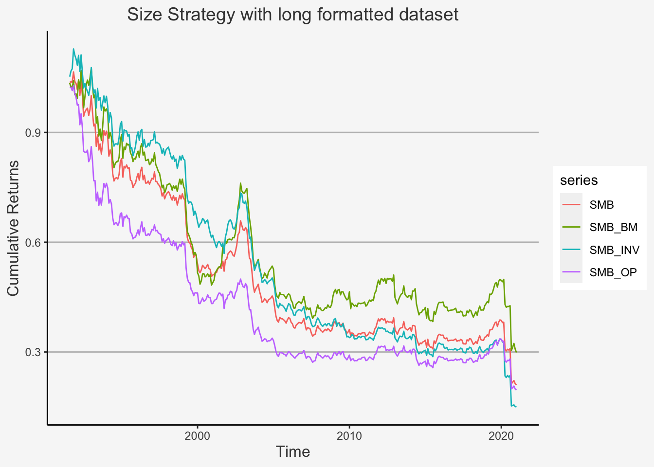
As we can see, the SMB factor has declining cumulative returns throughout time, implying that there appears to be no market anomaly related to this specific factor.
Finally, let’s calculate the summary statistics
# Calculate the three performance metrics
Annualised_Mean_Return <- Return.annualized(SMB)
Annualised_SD <- sd.annualized(SMB)
Sharpe_Ratio <- Annualised_Mean_Return/Annualised_SD

# Put it together
df_SMB <- as.data.frame(rbind(Annualised_Mean_Return, Annualised_SD, Sharpe_Ratio))
rownames(df_SMB) <- c("Annualised Return", "Standard Deviation", "Sharpe Ratio")

df_SMB
## SMB_BM SMB_OP SMB_INV SMB
## Annualised Return -0.03587035 -0.05180128 -0.05900121 -0.04904802
## Standard Deviation 0.11646017 0.10833291 0.11875724 0.10969154
## Sharpe Ratio -0.30800529 -0.47816754 -0.49682205 -0.447144986.5.5.2 High Minus Low, Robust Minus Weak and Conservative Minus Aggressive
Having created the SMB factor, let’s now replicate the HML, RMW as well as CMA factors. We will follow the same approach as Fama and French here again.
# Load the old dataset for book value
Book <- read.csv("~/Desktop/Master UZH/Data/A4_dataset_02_Ex_Session.txt", header = T, sep = "\t")
Book_check <- Book %>%
  gather(Ticker,value,NESN:X692395) %>%
  mutate(Date_t = lubridate::ceiling_date(dmy(Date), "month") - 1) %>%
  select(-Date)

colnames(Book_check) <- c("Ticker", "Total_Eq_Real", "Date_t")

# Only sub select the companies under consideration
tic_sub <- unique(names(read.csv("~/Desktop/Master UZH/Data/A4_dataset_04_Ex_Session.txt", header = T, sep = "\t")))

# Get 347 companies
CH_data_total_monthly <- read.csv("~/Desktop/CH_data_total_monthly.csv", header = T, sep = ",")
CH_data_total_monthly_clean <- CH_data_total_monthly[!duplicated(CH_data_total_monthly[c("Date_t", "Ticker")]),]

# Only get the respective columns
CH_data_total_mont <- CH_data_total_monthly_clean %>%
  subset(Ticker %in% tic_sub) %>%
  select(Date_t, Ticker, Adj_Close, Close, Num_Shares, Total_Eq_t, Gross_Inc_t, Operating_Exp_t, Interest_Exp_t, Total_Assets_t, Total_Liab_t) %>%
  mutate(Total_Eq_t = Total_Assets_t - Total_Liab_t,
         Num_Shares = Num_Shares,
         Date_t = as.Date(Date_t)) %>%
  group_by(Ticker) %>%
  mutate(Close = lag(Close, n=1),
         Num_Shares = lag(Num_Shares, 1)) %>%
  ungroup()


CH_data_total_mont_check <- left_join(CH_data_total_mont, Book_check, by = c("Ticker" = "Ticker", "Date_t" = "Date_t"))

# Control for extreme values
CH_data_total_monthly_sub_Size <- CH_data_total_mont_check %>%
  arrange(Date_t)  %>%
  group_by(Ticker) %>%
  mutate(Ret_Adj = (Adj_Close - lag(Adj_Close, 1))/lag(Adj_Close,1)) %>%
  na.omit() %>%
  ungroup() %>%
  group_by(Date_t) %>%
  mutate(Extreme_Values = quantile(Ret_Adj, p = 1),
         Extreme_Indicator = ifelse(Ret_Adj <= Extreme_Values, 1, NA),
         Ret_Adj = Ret_Adj * Extreme_Indicator) %>%
  ungroup()

# Create the variables for Size and Value
CH_data_total_monthly_sub_cumret_Size_Value <- CH_data_total_monthly_sub_Size %>%
  group_by(Ticker) %>%
  mutate(# Create the Market Cap (Size) characteristic
         Shares_Out_lagged = lag(Num_Shares, n = 1),
         Price_close_lagged = lag(Close, n = 1),
         Market_Cap = Shares_Out_lagged * Price_close_lagged,
         # Create the B2M (Value) characteristic
         Total_Eq_t = Total_Assets_t - Total_Liab_t,
         B2M = lag(Total_Eq_t, n = 6) / Market_Cap) %>%
  na.omit() %>%
  ungroup()

# Create the variables for Size and old Value
CH_data_total_monthly_sub_cumret_Size_Value_old <- CH_data_total_monthly_sub_Size %>%
  group_by(Ticker) %>%
  mutate(# Create the Market Cap (Size) characteristic
         Shares_Out_lagged = lag(Num_Shares, n = 1),
         Price_close_lagged = lag(Close, n = 1),
         Market_Cap = Shares_Out_lagged * Price_close_lagged,
         # Create the B2M (Value) characteristic
         B2M_old = lag(Total_Eq_Real, n = 6) / Market_Cap) %>%
  na.omit() %>%
  ungroup()

# Create the variables for Size and Operating Profitability
CH_data_total_monthly_sub_cumret_Size_Profit <- CH_data_total_monthly_sub_Size %>%
  group_by(Ticker) %>%
  mutate(# Create the Market Cap (Size) characteristic
         Shares_Out_lagged = lag(Num_Shares, n = 1),
         Price_close_lagged = lag(Close, n = 1),
         Market_Cap = Shares_Out_lagged * Price_close_lagged,
         # Create the B2M (Value) characteristic
         Profit_lead = (Gross_Inc_t - Operating_Exp_t - Interest_Exp_t)/Total_Eq_t,
         Profit = lag(Profit_lead, n = 1)) %>%
  na.omit() %>%
  ungroup()

# Create the variables for Size and Investment Growth
CH_data_total_monthly_sub_cumret_Size_Invest <- CH_data_total_monthly_sub_Size %>%
  group_by(Ticker) %>%
  mutate(# Create the Market Cap (Size) characteristic
         Shares_Out_lagged = lag(Num_Shares, n = 1),
         Price_close_lagged = lag(Close, n = 1),
         Market_Cap = Shares_Out_lagged * Price_close_lagged,
         # Create the B2M (Value) characteristic
         Invest_lead = (lag(Total_Assets_t, n =1) - lag(Total_Assets_t, n = 12))/lag(Total_Assets_t, n = 12),
         Invest = lag(Invest_lead, n = 1)) %>%
  na.omit() %>%
  ungroup()

# Assign Rankings for Size and Value
CH_data_total_monthly_sub_rank_Size_Value <- CH_data_total_monthly_sub_cumret_Size_Value %>%
  group_by(Date_t) %>%
  # Here we form the groups (ranks)
  mutate(# Create Small and Big Rank
          Size_Ranks = as.numeric(cut(Market_Cap,
               breaks = quantile(Market_Cap,
                                 probs= 0:2/2,
                                 na.rm = TRUE,
                                 type = 4),
               include.lowest = TRUE)),
         # Create Terciles based on B2M (Low, Neutral, High)
         Ranks = as.numeric(cut(B2M,
               breaks = quantile(B2M,
                                 probs= seq(0, 1, length = 11),
                                 na.rm = TRUE,
                                 type = 4),
               include.lowest = TRUE)),
         Value_Ranks = ifelse(Ranks <= 3, 1,
                              ifelse(Ranks > 3 & Ranks <= 7, 2,
                                     ifelse(Ranks > 7, 3, 0)))
         ) %>%
  ungroup()

# Assign Rankings for Size and Old Value
CH_data_total_monthly_sub_rank_Size_Value_old <- CH_data_total_monthly_sub_cumret_Size_Value_old %>%
  group_by(Date_t) %>%
  # Here we form the groups (ranks)
  mutate(# Create Small and Big Rank
          Size_Ranks = as.numeric(cut(Market_Cap,
               breaks = quantile(Market_Cap,
                                 probs= 0:2/2,
                                 na.rm = TRUE,
                                 type = 4),
               include.lowest = TRUE)),
         # Create Terciles based on B2M (Low, Neutral, High)
         Ranks = as.numeric(cut(B2M_old,
               breaks = quantile(B2M_old,
                                 probs= seq(0, 1, length = 11),
                                 na.rm = TRUE,
                                 type = 4),
               include.lowest = TRUE)),
         Value_old_Ranks = ifelse(Ranks <= 3, 1,
                              ifelse(Ranks > 3 & Ranks <= 7, 2,
                                     ifelse(Ranks > 7, 3, 0)))
         ) %>%
  ungroup()

# Assign Rankings for Size and Operating Profitability
CH_data_total_monthly_sub_rank_Size_Profit <- CH_data_total_monthly_sub_cumret_Size_Profit %>%
  group_by(Date_t) %>%
  # Here we form the groups (ranks)
  mutate(# Create Small and Big Rank
          Size_Ranks = as.numeric(cut(Market_Cap,
               breaks = quantile(Market_Cap,
                                 probs= 0:2/2,
                                 na.rm = TRUE,
                                 type = 4),
               include.lowest = TRUE)),
         # Create Terciles based on Oper Profit (Low, Neutral, High)
         Ranks = as.numeric(cut(Profit,
               breaks = quantile(Profit,
                                 probs= seq(0, 1, length = 11),
                                 na.rm = TRUE,
                                 type = 4),
               include.lowest = TRUE)),
         Profit_Ranks = ifelse(Ranks <= 3, 1,
                              ifelse(Ranks > 3 & Ranks <= 7, 2,
                                     ifelse(Ranks > 7, 3, 0)))
         ) %>%
  ungroup()

# Assign Rankings for Size and Investment Growth
CH_data_total_monthly_sub_rank_Size_Invest <- CH_data_total_monthly_sub_cumret_Size_Invest %>%
  group_by(Date_t) %>%
  # Here we form the groups (ranks)
  mutate(# Create Small and Big Rank
          Size_Ranks = as.numeric(cut(Market_Cap,
               breaks = quantile(Market_Cap,
                                 probs= 0:2/2,
                                 na.rm = TRUE,
                                 type = 4),
               include.lowest = TRUE)),
         # Create Terciles based on Investment Growth (Low, Neutral, High)
         Ranks = ntile(Total_Assets_t, 10),
         Invest_Ranks = ifelse(Ranks <= 3, 1,
                              ifelse(Ranks > 3 & Ranks <= 7, 2,
                                     ifelse(Ranks > 7, 3, 0)))
         ) %>%
  ungroup()


# Create the average returns per group for Size and Value
CH_data_EW_Ret_HML <- CH_data_total_monthly_sub_rank_Size_Value %>%
  group_by(Date_t, Size_Ranks, Value_Ranks) %>%
  mutate(EW_Ret_mean_t_Size_Value = mean(Ret_Adj, na.rm = T),
         EW_Ret_sd_t_Size_Value = sd(Ret_Adj, na.rm = T)) %>%
    select(Date_t,Size_Ranks, Value_Ranks, EW_Ret_mean_t_Size_Value,EW_Ret_sd_t_Size_Value) %>%
  ungroup() %>%
  unique() %>%
  arrange(Date_t,Size_Ranks, Value_Ranks) %>%
  group_by(Date_t, Value_Ranks) %>%
  mutate(High_Size = ifelse(Value_Ranks == 3, mean(EW_Ret_mean_t_Size_Value), 0),
         Low_Size = ifelse(Value_Ranks == 1, mean(EW_Ret_mean_t_Size_Value), 0)) %>%
  ungroup() %>%
  select(Date_t, High_Size, Low_Size) %>%
  unique() %>%
  group_by(Date_t) %>%
  mutate(HML = sum(High_Size) - sum(Low_Size)) %>%
  select(Date_t, HML) %>%
  unique()

# Create the average returns per group for Size and Old Value
CH_data_EW_Ret_HML_old <- CH_data_total_monthly_sub_rank_Size_Value_old %>%
  group_by(Date_t, Size_Ranks, Value_old_Ranks) %>%
  mutate(EW_Ret_mean_t_Size_Value_old = mean(Ret_Adj, na.rm = T),
         EW_Ret_sd_t_Size_Value_old = sd(Ret_Adj, na.rm = T)) %>%
    select(Date_t,Size_Ranks, Value_old_Ranks, EW_Ret_mean_t_Size_Value_old,EW_Ret_sd_t_Size_Value_old) %>%
  ungroup() %>%
  unique() %>%
  arrange(Date_t,Size_Ranks, Value_old_Ranks) %>%
  group_by(Date_t, Value_old_Ranks) %>%
  mutate(High_Size = ifelse(Value_old_Ranks == 3, mean(EW_Ret_mean_t_Size_Value_old), 0),
         Low_Size = ifelse(Value_old_Ranks == 1, mean(EW_Ret_mean_t_Size_Value_old), 0)) %>%
  ungroup() %>%
  select(Date_t, High_Size, Low_Size) %>%
  unique() %>%
  group_by(Date_t) %>%
  mutate(HML_old = sum(High_Size) - sum(Low_Size)) %>%
  select(Date_t, HML_old) %>%
  unique()

# Create the average returns per group for Size and Operating Profitability
CH_data_EW_Ret_Size_RMW <- CH_data_total_monthly_sub_rank_Size_Profit %>% group_by(Date_t, Size_Ranks, Profit_Ranks) %>%
  mutate(EW_Ret_mean_t_Size_Profit = mean(Ret_Adj, na.rm = T),
         EW_Ret_sd_t_Size_Profit = sd(Ret_Adj, na.rm = T)) %>%
    select(Date_t,Size_Ranks, Profit_Ranks, EW_Ret_mean_t_Size_Profit,EW_Ret_sd_t_Size_Profit) %>%
  ungroup() %>%
  unique() %>%
  arrange(Date_t,Size_Ranks, Profit_Ranks) %>%
  group_by(Date_t, Profit_Ranks) %>%
  mutate(Robust_Size = ifelse(Profit_Ranks == 3, mean(EW_Ret_mean_t_Size_Profit), 0),
         Weak_Size = ifelse(Profit_Ranks == 1, mean(EW_Ret_mean_t_Size_Profit), 0)) %>%
  ungroup() %>%
  select(Date_t, Robust_Size, Weak_Size) %>%
  unique() %>%
  group_by(Date_t) %>%
  mutate(RMW = sum(Robust_Size) - sum(Weak_Size)) %>%
  select(Date_t, RMW) %>%
  unique()

# Create the average returns per group for Size and Investment Growth
CH_data_EW_Ret_CMA <- CH_data_total_monthly_sub_rank_Size_Invest %>% group_by(Date_t, Size_Ranks, Invest_Ranks) %>%
  mutate(EW_Ret_mean_t_Size_Invest = mean(Ret_Adj, na.rm = T),
         EW_Ret_sd_t_Size_Invest = sd(Ret_Adj, na.rm = T)) %>%
    select(Date_t,Size_Ranks, Invest_Ranks, EW_Ret_mean_t_Size_Invest,EW_Ret_sd_t_Size_Invest) %>%
  ungroup() %>%
  unique() %>%
  arrange(Date_t,Size_Ranks, Invest_Ranks) %>%
  group_by(Date_t, Invest_Ranks) %>%
  mutate(Aggressive_Ranks = ifelse(Invest_Ranks == 3, mean(EW_Ret_mean_t_Size_Invest), 0),
         Conservative_Ranks = ifelse(Invest_Ranks == 1, mean(EW_Ret_mean_t_Size_Invest), 0)) %>%
  ungroup() %>%
  select(Date_t, Aggressive_Ranks, Conservative_Ranks) %>%
  unique() %>%
  group_by(Date_t) %>%
  mutate(CMA = sum(Conservative_Ranks) - sum(Aggressive_Ranks)) %>%
  select(Date_t, CMA) %>%
  unique()

# Combine the three individual factors
## Create three xts objects
CH_data_EW_Ret_HML_ts <- xts(CH_data_EW_Ret_HML[,-1], order.by = as.Date(CH_data_EW_Ret_HML$Date_t))
CH_data_EW_Ret_HML_old_ts <- xts(CH_data_EW_Ret_HML_old[,-1], order.by = as.Date(CH_data_EW_Ret_HML_old$Date_t))
CH_data_EW_Ret_Size_RMW_ts <- xts(CH_data_EW_Ret_Size_RMW[,-1], order.by = as.Date(CH_data_EW_Ret_Size_RMW$Date_t))
CH_data_EW_Ret_Size_CMA_ts <- xts(CH_data_EW_Ret_CMA[,-1], order.by = as.Date(CH_data_EW_Ret_CMA$Date_t))

Factors <- merge.xts(SMB$SMB, CH_data_EW_Ret_HML_ts, CH_data_EW_Ret_Size_RMW_ts, CH_data_EW_Ret_Size_CMA_ts)


cumprod(1+na.omit(Factors["1991-02-28/2020-12-31"])) %>% tidy() %>% ggplot(aes(x =index ,y = value ,color = series)) +
    geom_line( size = 0.5 ) +
    ggtitle("Size, Value, Profitability and Investment Growth Strategy") +
  ylab("Cumulative Returns") + xlab("Time") +
theme(plot.title= element_text(size=14, color="grey26",
hjust=0.5,
lineheight=1.2), panel.background = element_rect(fill="#f7f7f7"),
panel.grid.major.y = element_line(size = 0.5, linetype = "solid", color = "grey"),
panel.grid.minor = element_blank(),
panel.grid.major.x = element_blank(),
plot.background = element_rect(fill="#f7f7f7", color = "#f7f7f7"), axis.title.x = element_text(color="grey26", size=12),
axis.title.y = element_text(color="grey26", size=12),
axis.line = element_line(color = "black")) 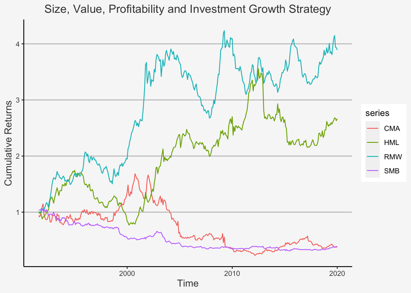
As we can see, the Profitability factor appears to be the strongest anomaly of the factors under consideration. The value factor also shows significant, positive, albeit less pronounced, returns for the period under consideration. On the other hand, both the Investment as well as the size factor appear to be no material anomaly in the Swiss market from the observational time horizon.
Finally, let’s calculate the summary statistics
# Calculate the three performance metrics
Annualised_Mean_Return <- Return.annualized(Factors)
Annualised_SD <- sd.annualized(Factors)
Sharpe_Ratio <- Annualised_Mean_Return/Annualised_SD

# Put it together
df_factors <- as.data.frame(rbind(Annualised_Mean_Return, Annualised_SD, Sharpe_Ratio))
rownames(df_factors) <- c("Annualised Return", "Standard Deviation", "Sharpe Ratio")

df_factors
## SMB HML RMW CMA
## Annualised Return -0.04904802 0.0331400 0.05414061 -0.03357213
## Standard Deviation 0.10969154 0.1285831 0.10801873 0.19642474
## Sharpe Ratio -0.44714498 0.2577321 0.50121499 -0.170916026.5.5.3 Up Minus Down
Lastly, we will show you the performance of the Momentum factor, or UMD. We will create the factor based on both the Jegadeesh and Titman (1995) approach (the original approach of their paper) as well as the more static approach used by Carharrt (1996).
We will first create the approach of Carharrt (1996).
# Load the old datasets for check up
Prices_Adj <- read.csv("~/Desktop/Master UZH/Data/A4_dataset_01_Ex_Session.txt", header = T, sep = "\t")

Prices_Unadj_check <- Prices_Adj %>%
  gather(Ticker,value,NESN:X692395) %>%
  mutate(Date_t = lubridate::ceiling_date(dmy(Date), "month") - 1) %>%
  select(-Date)

colnames(Prices_Unadj_check) <- c("Ticker", "Close_Real", "Date_t")

# Get only selected companies
tic_sub <- unique(names(read.csv("~/Desktop/Master UZH/Data/A4_dataset_04_Ex_Session.txt", header = T, sep = "\t")))

# Get 347 companies
CH_data_total_monthly <- read.csv("~/Desktop/CH_data_total_monthly.csv", header = T, sep = ",")
CH_data_total_monthly_clean <- CH_data_total_monthly[!duplicated(CH_data_total_monthly[c("Date_t", "Ticker")]),]

# Only get the respective columns
CH_data_total_mont <- CH_data_total_monthly_clean %>%
  subset(Ticker %in% tic_sub) %>%
  select(Date_t, Ticker, Adj_Close, Close, Num_Shares, Total_Eq_t, Gross_Inc_t, Operating_Exp_t, Interest_Exp_t, Total_Assets_t) %>%
  mutate(Total_Eq_t = Total_Eq_t,
         Num_Shares = Num_Shares,
         Date_t = as.Date(Date_t)) %>%
  group_by(Ticker) %>%
  mutate(Close = lag(Close, n=1),
         Total_Eq_t = lag(Total_Eq_t, 1),
         Num_Shares = lag(Num_Shares, 1)) %>%
  ungroup()


CH_data_total_mont_check <- left_join(CH_data_total_mont, Prices_Unadj_check, by = c("Ticker" = "Ticker", "Date_t" = "Date_t"))

# Control for extreme values
CH_data_total_monthly_sub_Size <- CH_data_total_mont_check %>%
  arrange(Date_t)  %>%
  group_by(Ticker) %>%
  mutate(Ret_Adj = (Adj_Close - lag(Adj_Close, 1))/lag(Adj_Close,1),
         Ret_Adj_old = (Close_Real - lag(Close_Real, 1))/lag(Close_Real,1)) %>%
  na.omit() %>%
  ungroup() %>%
  group_by(Date_t) %>%
  mutate(Extreme_Values = quantile(Ret_Adj, p = 1),
         Extreme_Indicator = ifelse(Ret_Adj <= Extreme_Values, 1, NA),
         Ret_Adj = Ret_Adj * Extreme_Indicator) %>%
  ungroup()


# Create the variables for Size and Momentum
CH_data_total_monthly_sub_cumret_Size_Mom <- CH_data_total_monthly_sub_Size %>%
  group_by(Ticker) %>%
  mutate(# Create the Market Cap (Size) characteristic
         Shares_Out_lagged = lag(Num_Shares, n = 1),
         Price_close_lagged = lag(Close, n = 1),
         Market_Cap = Shares_Out_lagged * Price_close_lagged,
         # Create the Cumulative Returns (Momentum) characteristic
         Log_Ret_Adj = lag(log(1+Ret_Adj), n = 1),
         Sum_Ret = roll_sum(Log_Ret_Adj, 6),
         Cum_Ret = exp(Sum_Ret) - 1,
         ) %>%
  na.omit() %>%
  ungroup()

# Assign Rankings for Size and Momentum
CH_data_total_monthly_sub_rank_Size_Mom <- CH_data_total_monthly_sub_cumret_Size_Mom %>%
  group_by(Date_t) %>%
  # Here we form the groups (ranks)
  mutate(# Create Small and Big Rank
          Size_Ranks = as.numeric(cut(Market_Cap,
               breaks = quantile(Market_Cap,
                                 probs= 0:2/2,
                                 na.rm = TRUE,
                                 type = 4),
               include.lowest = TRUE)),
         # Create Terciles based on B2M (Low, Neutral, High)
         Ranks = as.numeric(cut(Cum_Ret,
               breaks = quantile(Cum_Ret,
                                 probs= seq(0, 1, length = 11),
                                 na.rm = TRUE,
                                 type = 4),
               include.lowest = TRUE)),
         Mom_Ranks = ifelse(Ranks <= 3, 1,
                              ifelse(Ranks > 3 & Ranks <= 7, 2,
                                     ifelse(Ranks > 7, 3, 0)))
         ) %>%
  ungroup()

# Create the average returns per group for Size and Momentum
CH_data_EW_Ret_Mom <- CH_data_total_monthly_sub_rank_Size_Mom %>%
  group_by(Date_t, Size_Ranks, Mom_Ranks) %>%
  mutate(EW_Ret_mean_t_Size_Mom = mean(Ret_Adj, na.rm = T),
         EW_Ret_sd_t_Size_Mom = sd(Ret_Adj, na.rm = T)) %>%
    select(Date_t,Size_Ranks, Mom_Ranks, EW_Ret_mean_t_Size_Mom,EW_Ret_sd_t_Size_Mom) %>%
  ungroup() %>%
  unique() %>%
  arrange(Date_t,Size_Ranks, Mom_Ranks) %>%
  group_by(Date_t, Mom_Ranks) %>%
  mutate(Up_Size = ifelse(Mom_Ranks == 3, mean(EW_Ret_mean_t_Size_Mom), 0),
         Down_Size = ifelse(Mom_Ranks == 1, mean(EW_Ret_mean_t_Size_Mom), 0)) %>%
  ungroup() %>%
  select(Date_t, Up_Size, Down_Size) %>%
  unique() %>%
  group_by(Date_t) %>%
  mutate(MOM = sum(Up_Size) - sum(Down_Size)) %>%
  select(Date_t, MOM) %>%
  unique()

colnames(CH_data_EW_Ret_Mom) <- c("Date_t", "Momentum_Car")

# Combine the three individual factors
## Create the xts objects
CH_data_EW_Ret_MOM_ts <- xts(CH_data_EW_Ret_Mom[,-1], order.by = as.Date(CH_data_EW_Ret_Mom$Date_t))
Now, we will replicate the approach of Jegadeesh and Titman (1995).
# Let's run the experiment for the reduced data frame
tic_sub <- unique(names(read.csv("~/Desktop/Master UZH/Data/A4_dataset_04_Ex_Session.txt", header = T, sep = "\t")))
# Get 347 companies
CH_data_total_monthly <- read.csv("~/Desktop/CH_data_total_monthly.csv", header = T, sep = ",")
CH_data_total_monthly_clean <- CH_data_total_monthly[!duplicated(CH_data_total_monthly[c("Date_t", "Ticker")]),]

# Only get the respective columns
CH_data_total_mont <- CH_data_total_monthly_clean %>%
  subset(Ticker %in% tic_sub) %>%
  select(Date_t, Ticker, Adj_Close,  Num_Shares, Close) %>%
  mutate(Date_t = as.Date(Date_t),
         Date_t = as.yearmon(Date_t))

# Control for extreme values
CH_data_total_monthly_sub <- CH_data_total_mont %>%
  arrange(Date_t) %>%
  select(Date_t, Ticker, Adj_Close, Num_Shares, Close) %>%
  group_by(Ticker) %>%
  mutate(Ret_Adj = (Adj_Close - lag(Adj_Close, 1))/lag(Adj_Close,1)) %>%
  na.omit() %>%
  ungroup() %>%
  group_by(Date_t) %>%
  mutate(Extreme_Values = quantile(Ret_Adj, p = 1),
         Extreme_Indicator = ifelse(Ret_Adj <= Extreme_Values, 1, NA),
         Ret_Adj = Ret_Adj * Extreme_Indicator) %>%
  ungroup()

# Get the lagged values to ensure that we have a HPR of 6 periods!
# Since we go 6 periods behind and take the cum ret from period -6 to period -1 to obtain the HPR from period -5 to 0.

# Idea: If we do it like this, we account for gaps in the data. E.g. if two observational periods were on Aug 1990 and then on Aug 1991, the gap would be 12 periods. Thus, this would not constitute a HPR of 6 periods, but 12. In order to ensure we only ever get HPR of 6 periods, we need to create the indicator which shows how many periods (in months) two dates are apart from one another. This must equal 6 and not more!

CH_data_total_monthly_sub_lag <- CH_data_total_monthly_sub %>%
  group_by(Ticker) %>%
  mutate(lag6 = round(12*(Date_t - lag(Date_t, n=5)))/5)

# Get the adjustred returns to form the PF on
CH_data_total_monthly_sub_cumret <- CH_data_total_monthly_sub_lag %>%
  group_by(Ticker) %>%
  mutate(Shares_Out_lagged = lag(Num_Shares, n = 1),
         Price_close_lagged = lag(Close, n = 1),
         Market_Cap = Shares_Out_lagged * Price_close_lagged,
         # Create the Cumulative Returns (Momentum) characteristic
         Log_Ret_Adj = lag(log(1+Ret_Adj), n = 1),
         Sum_Ret = roll_sum(Log_Ret_Adj, 6),
         Cum_Ret = exp(Sum_Ret) - 1) %>%
  na.omit() %>%
  ungroup()

# Assign Rankings for Size and Momentum
CH_data_total_monthly_sub_rank_lag <- CH_data_total_monthly_sub_cumret %>%
  group_by(Date_t) %>%
  # Here we form the groups (ranks)
  mutate(# Create Small and Big Rank
          Size_Ranks = as.numeric(cut(Market_Cap,
               breaks = quantile(Market_Cap,
                                 probs= 0:2/2,
                                 na.rm = TRUE,
                                 type = 4),
               include.lowest = TRUE)),
         # Create Terciles based on B2M (Low, Neutral, High)
         Ranks = as.numeric(cut(Cum_Ret,
               breaks = quantile(Cum_Ret,
                                 probs= seq(0, 1, length = 11),
                                 na.rm = TRUE,
                                 type = 4),
               include.lowest = TRUE)),
         Mom_Ranks = ifelse(Ranks <= 3, 1,
                              ifelse(Ranks > 3 & Ranks <= 7, 2,
                                     ifelse(Ranks > 7, 3, 0)))
         ) %>%
  ungroup()

# Select only certain columns
CH_data_total_monthly_sub_rank_2_lag <- CH_data_total_monthly_sub_rank_lag %>%
  select(Date_t, Ticker, Mom_Ranks, Size_Ranks)

# Create the average returns per group for Size and Momentum
CH_data_total_monthly_sub_rank_tot <- CH_data_total_monthly_sub_lag %>% ungroup() %>%
    filter(., lag6 == 1 ) %>%
    left_join(CH_data_total_monthly_sub_rank_2_lag, by = c("Ticker"="Ticker", "Date_t" = "Date_t")) %>%
    select(Ticker,Date_t,Ret_Adj,Mom_Ranks, Size_Ranks) %>%
    arrange(Ticker,Date_t) %>%
    group_by(Date_t,Mom_Ranks) %>%
    mutate(momr = mean(Ret_Adj, na.rm = T)) %>% ungroup() %>%
    select(Date_t,Mom_Ranks,Size_Ranks, momr) %>%
    ungroup()  %>%
    unique() %>%
    arrange(Date_t,Size_Ranks, Mom_Ranks) %>%
    group_by(Date_t, Mom_Ranks) %>%
    mutate(Up_Size = ifelse(Mom_Ranks == 3, mean(momr), 0),
           Down_Size = ifelse(Mom_Ranks == 1, mean(momr), 0)) %>%
    ungroup() %>%
    select(Date_t, Up_Size, Down_Size) %>%
    unique() %>%
    group_by(Date_t) %>%
    mutate(MOM = sum(Up_Size, na.rm = T) - sum(Down_Size, na.rm = T),
           Date_t = lubridate::ceiling_date(my(Date_t), "month") - 1) %>%
    select(Date_t, MOM) %>%
    unique()

colnames(CH_data_total_monthly_sub_rank_tot) <- c("Date_t", "Momentum_JT")

# Combine the three individual factors
## Create the xts objects
CH_data_EW_Ret_MOM_JT_ts <- xts(CH_data_total_monthly_sub_rank_tot[,-1], order.by = as.Date(CH_data_total_monthly_sub_rank_tot$Date_t))
Now, we can combine both approaches and see the differences in cumulative returns.
# Create a merged xts object
Factors <- merge.xts(CH_data_EW_Ret_MOM_ts, CH_data_EW_Ret_MOM_JT_ts)

# Plot the relationship
cumprod(1+na.omit(Factors["1991-02-28/2020-12-31"])) %>% tidy() %>% ggplot(aes(x =index ,y = value ,color = series)) +
    geom_line( size = 0.5 ) +
    ggtitle("Momentum Strategies") +
  ylab("Cumulative Returns") + xlab("Time") +
theme(plot.title= element_text(size=14, color="grey26",
hjust=0.5,
lineheight=1.2), panel.background = element_rect(fill="#f7f7f7"),
panel.grid.major.y = element_line(size = 0.5, linetype = "solid", color = "grey"),
panel.grid.minor = element_blank(),
panel.grid.major.x = element_blank(),
plot.background = element_rect(fill="#f7f7f7", color = "#f7f7f7"), axis.title.x = element_text(color="grey26", size=12),
axis.title.y = element_text(color="grey26", size=12),
axis.line = element_line(color = "black")) 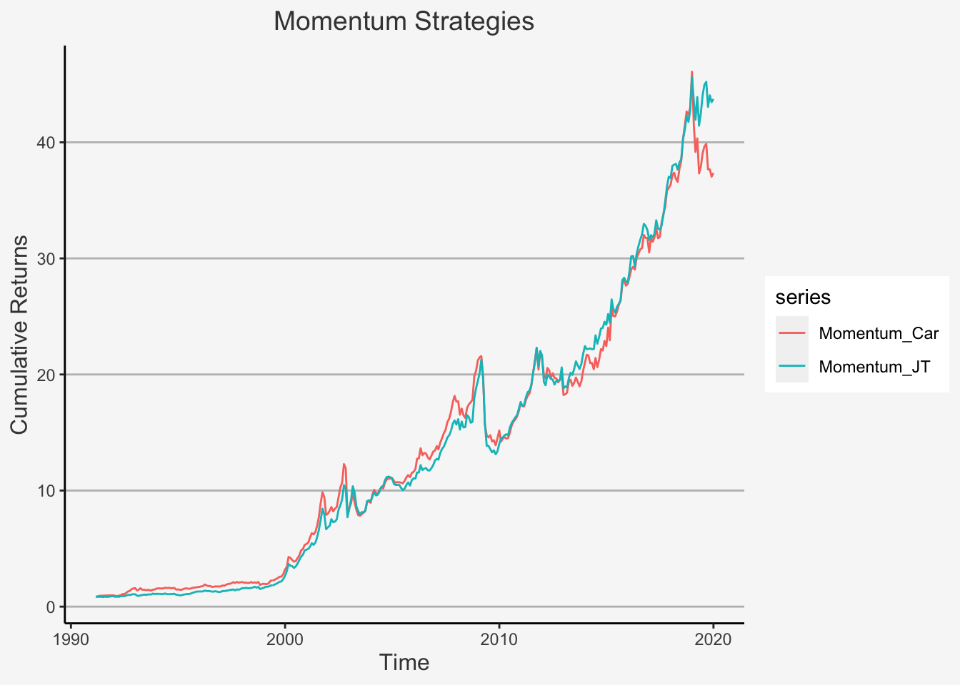
As we can see, there are slight differences in the cumulative return structures of both strategies, whereas it appears as if the factor construction of Jegadeesh and Titman (JT) delivers, on average, higher cumulative returns, especially after 2012.
Finally, let’s calculate the summary statistics
# Calculate the three performance metrics
Annualised_Mean_Return <- Return.annualized(Factors)
Annualised_SD <- sd.annualized(Factors)
Sharpe_Ratio <- Annualised_Mean_Return/Annualised_SD

# Put it together
df_MOM <- as.data.frame(rbind(Annualised_Mean_Return, Annualised_SD, Sharpe_Ratio))
rownames(df_MOM) <- c("Annualised Return", "Standard Deviation", "Sharpe Ratio")

df_MOM
## Momentum_Car Momentum_JT
## Annualised Return 0.1327952 0.1587250
## Standard Deviation 0.1716485 0.1797972
## Sharpe Ratio 0.7736459 0.88280046.5.5.4 Betting Against Beta
# Let's run the experiment for the reduced data frame
tic_sub <- unique(names(read.csv("~/Desktop/Master UZH/Data/A4_dataset_04_Ex_Session.txt", header = T, sep = "\t")))
# Get 347 companies
CH_data_total_monthly <- read.csv("~/Desktop/CH_data_total_monthly.csv", header = T, sep = ",")
CH_data_total_monthly_clean <- CH_data_total_monthly[!duplicated(CH_data_total_monthly[c("Date_t", "Ticker")]),]

# Only get the respective columns
CH_data_total_mont <- CH_data_total_monthly_clean %>%
  subset(Ticker %in% tic_sub) %>%
  select(Date_t, Ticker, Adj_Close, Total_Assets_t)

# Control for extreme values
CH_data_total_monthly_sub_BAB <- CH_data_total_mont %>%
  arrange(Date_t)  %>%
  group_by(Ticker) %>%
  mutate(Ret_Adj = (Adj_Close - lag(Adj_Close, 1))/lag(Adj_Close,1)) %>%
  na.omit() %>%
  ungroup() %>%
  group_by(Date_t) %>%
  mutate(Extreme_Values = quantile(Ret_Adj, p = 1),
         Extreme_Indicator = ifelse(Ret_Adj <= Extreme_Values, 1, NA),
         Ret_Adj = Ret_Adj * Extreme_Indicator) %>%
  ungroup()


# Let's also get the data on the Swiss Market Index as well as the risk free rate
rf <- read.csv("~/Desktop/Master UZH/Data/A2_dataset_02_Ex_Session.txt", header = T, sep = "\t")
rf_ts <- rf %>%
  subset((Date >= '1989-12-01') & (Date <= '2019-12-31')) %>%
  mutate(rf_annual = SWISS.CONFEDERATION.BOND.1.YEAR...RED..YIELD / 1000,
         rf_monthly =  (1 + rf_annual)^(1/12) - 1) %>%
  select(Date, rf_monthly)


SMI <-  read.csv("~/Desktop/Master UZH/Data/A2_dataset_03_Ex_Session.txt", header = T, sep = "\t")
SMI_ts <- SMI %>%
  subset((Date >= '1989-12-01') & (Date <= '2019-12-31')) %>%
  mutate(SMI_ret = (SMI - lag(SMI, 1))/lag(SMI, 1),
         rf_monthly = rf_ts$rf_monthly,
         SMI_rf_excess_ret = SMI_ret - rf_monthly)

# Now, let's calculate the excess returns
SMI_rf_ts_ret <- SMI_ts_ret - rf_ts_monthly
CH_data_total_monthly_sub_excess_ret_BAB <- left_join(SMI_ts, CH_data_total_monthly_sub_BAB, by = c("Date" = "Date_t")) %>%
  mutate(Excess_Ret_Adj = Ret_Adj - rf_monthly)

# Based on this, we can now have rolling regressions of the correlation as well as the standard deviations.
CH_data_total_monthly_weighted_BAB <- CH_data_total_monthly_sub_excess_ret_BAB %>%
  group_by(Ticker) %>%
  mutate(sd_roll_1_year = roll_sd(Excess_Ret_Adj, width = 12),
         corr_roll_5_year = roll_cor(Excess_Ret_Adj, SMI_rf_excess_ret, width = 60),
         sd_roll_1_year_Market = roll_sd(SMI_rf_excess_ret, width = 12),
         Beta_Est_raw = sd_roll_1_year/sd_roll_1_year_Market*corr_roll_5_year,
         Beta_Est_Adj = Beta_Est_raw*0.6 + 0.4*1) %>%
  ungroup() %>%
  subset(!is.na(Beta_Est_Adj)) %>%
  group_by(Date) %>%
  mutate(ranks_beta = rank(Beta_Est_Adj),
         mean_rank_beta = mean(ranks_beta, na.rm = T),
         portfolio_indicator_BAB =ifelse(ranks_beta > mean_rank_beta, 1, 0)) %>%
  ungroup() %>%
  group_by(Date, portfolio_indicator_BAB) %>%
  mutate(abs_dev = abs(ranks_beta - mean_rank_beta),
         sum_abs_dev = sum(abs_dev, na.rm = T),
         k = 2 / sum_abs_dev,
         weights_BAB = k*(ranks_beta - mean_rank_beta),
         Beta_Est_Weight_Adj = Beta_Est_Adj * weights_BAB) %>%
  ungroup()

# Assign rankings
CH_data_total_monthly_rank_BAB <- CH_data_total_monthly_weighted_BAB %>%
  group_by(Date) %>%
  mutate(Decile = ntile(Beta_Est_Weight_Adj, 2)) %>%
  ungroup()

# Create mean returns Decile
CH_data_EW_Ret_BAB <- CH_data_total_monthly_rank_BAB %>%
  group_by(Date, Decile) %>%
  mutate(EW_Ret_mean_t = 1/sum(Beta_Est_Weight_Adj)*sum(weights_BAB*Excess_Ret_Adj)) %>%
  select(Date, Decile, EW_Ret_mean_t) %>%
  ungroup() %>%
  unique() %>%
  arrange(Date, Decile) %>%
  spread(key = Decile, value = EW_Ret_mean_t) %>%
  mutate(BAB = `1` - `2`,
         BAB_cr = cumprod(1+BAB))

CH_data_EW_Ret_BAB %>%
ggplot() +
    geom_line(mapping = aes(x =as.Date(Date),y = BAB_cr), size = 0.5, color = "goldenrod") +
    ggtitle("BAB Strategy with long formatted dataset") +
  ylab("Cumulative Returns") + xlab("Time") +
theme(plot.title= element_text(size=14, color="grey26",
hjust=0.5,
lineheight=1.2), panel.background = element_rect(fill="#f7f7f7"),
panel.grid.major.y = element_line(size = 0.5, linetype = "solid", color = "grey"),
panel.grid.minor = element_blank(),
panel.grid.major.x = element_blank(),
plot.background = element_rect(fill="#f7f7f7", color = "#f7f7f7"), axis.title.x = element_text(color="grey26", size=12),
axis.title.y = element_text(color="grey26", size=12),
axis.line = element_line(color = "black")) 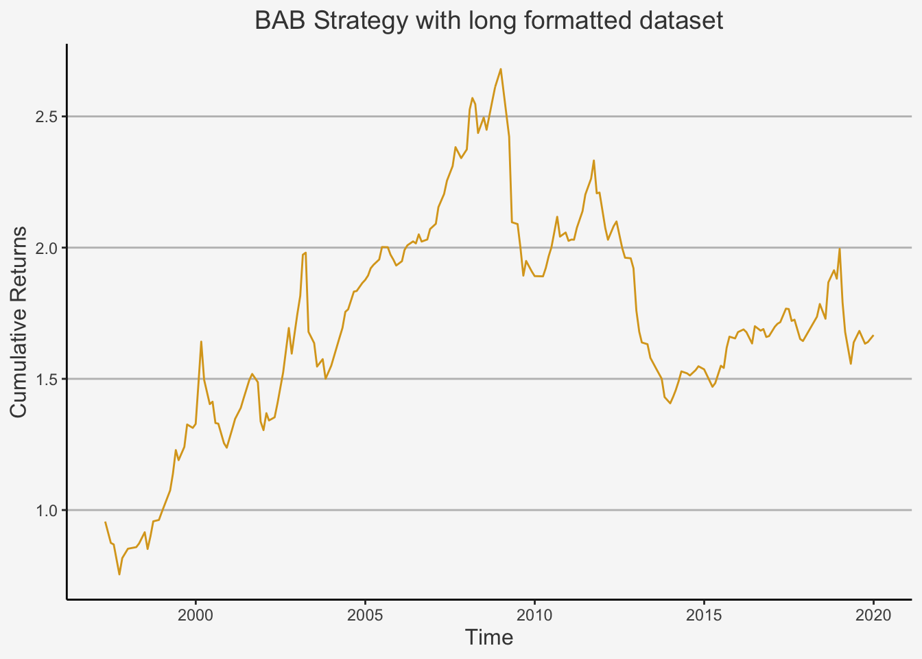
Finally, let’s calculate the summary statistics
CH_data_EW_Ret_BAB_ts <- xts(CH_data_EW_Ret_BAB$BAB, order.by = as.Date(CH_data_EW_Ret_BAB$Date))

# Calculate the three performance metrics
Annualised_Mean_Return <- Return.annualized(CH_data_EW_Ret_BAB_ts)
Annualised_SD <- sd.annualized(CH_data_EW_Ret_BAB_ts)
Sharpe_Ratio <- Annualised_Mean_Return/Annualised_SD

# Put it together
df_BAB<- as.data.frame(rbind(Annualised_Mean_Return, Annualised_SD, Sharpe_Ratio))
rownames(df_BAB) <- c("Annualised Return", "Standard Deviation", "Sharpe Ratio")
colnames(df_BAB) <- "BAB"

df_BAB
## BAB
## Annualised Return 0.03227748
## Standard Deviation 0.15029547
## Sharpe Ratio 0.214760186.5.6 The importance of data selection
We have now seen how to calculate five of the most widespread factors in asset management. Lastly, we deem it necessary to show you the importance of data accessibility. This follows the fact that identical databases provide different data based on the sub-section of the respective database. Since the data is different, the exactly identical approach to construct the factor at hand will, inadvertedly, lead to different end results. This should hightlight both the discrepancy of data availability and stress the need to always thoroughly double-check and cross-reference your data in order to circumvent the issue of incoherent data mining.
To do so, we retrieved data to calculate the Value factor from Thomson Reuters Datastream as well as Bloomberg, two of the largest data providers. We calculate the Value factor in an identical way and plot both cumulative returns to show the (substantial) differences when using different sets of data.
# Load the old dataset for book value
Book <- read.csv("~/Desktop/Master UZH/Data/A4_dataset_02_Ex_Session.txt", header = T, sep = "\t")
Book_check <- Book %>%
  gather(Ticker,value,NESN:X692395) %>%
  mutate(Date_t = lubridate::ceiling_date(dmy(Date), "month") - 1) %>%
  select(-Date)

colnames(Book_check) <- c("Ticker", "Total_Eq_Real", "Date_t")

# Only sub select the companies under consideration
tic_sub <- unique(names(read.csv("~/Desktop/Master UZH/Data/A4_dataset_04_Ex_Session.txt", header = T, sep = "\t")))

# Get 347 companies
CH_data_total_monthly <- read.csv("~/Desktop/CH_data_total_monthly.csv", header = T, sep = ",")
CH_data_total_monthly_clean <- CH_data_total_monthly[!duplicated(CH_data_total_monthly[c("Date_t", "Ticker")]),]

# Only get the respective columns
CH_data_total_mont <- CH_data_total_monthly_clean %>%
  subset(Ticker %in% tic_sub) %>%
  select(Date_t, Ticker, Adj_Close, Close, Num_Shares, Total_Eq_t, Gross_Inc_t, Operating_Exp_t, Interest_Exp_t, Total_Assets_t, Total_Liab_t) %>%
  mutate(Total_Eq_t = Total_Assets_t - Total_Liab_t,
         Num_Shares = Num_Shares,
         Date_t = as.Date(Date_t)) %>%
  group_by(Ticker) %>%
  mutate(Close = lag(Close, n=1),
         Num_Shares = lag(Num_Shares, 1)) %>%
  ungroup()


CH_data_total_mont_check <- left_join(CH_data_total_mont, Book_check, by = c("Ticker" = "Ticker", "Date_t" = "Date_t"))

# Control for extreme values
CH_data_total_monthly_sub_Size <- CH_data_total_mont_check %>%
  arrange(Date_t)  %>%
  group_by(Ticker) %>%
  mutate(Ret_Adj = (Adj_Close - lag(Adj_Close, 1))/lag(Adj_Close,1)) %>%
  na.omit() %>%
  ungroup() %>%
  group_by(Date_t) %>%
  mutate(Extreme_Values = quantile(Ret_Adj, p = 1),
         Extreme_Indicator = ifelse(Ret_Adj <= Extreme_Values, 1, NA),
         Ret_Adj = Ret_Adj * Extreme_Indicator) %>%
  ungroup()

# Create the variables for Size Value TR
CH_data_total_monthly_sub_cumret_Size_Value <- CH_data_total_monthly_sub_Size %>%
  group_by(Ticker) %>%
  mutate(# Create the Market Cap (Size) characteristic
         Shares_Out_lagged = lag(Num_Shares, n = 1),
         Price_close_lagged = lag(Close, n = 1),
         Market_Cap = Shares_Out_lagged * Price_close_lagged,
         # Create the B2M (Value) characteristic
         Total_Eq_t = Total_Assets_t - Total_Liab_t,
         B2M = lag(Total_Eq_t, n = 6) / Market_Cap) %>%
  na.omit() %>%
  ungroup()

# Create the variables for Size and Value BL
CH_data_total_monthly_sub_cumret_Size_Value_old <- CH_data_total_monthly_sub_Size %>%
  group_by(Ticker) %>%
  mutate(# Create the Market Cap (Size) characteristic
         Shares_Out_lagged = lag(Num_Shares, n = 1),
         Price_close_lagged = lag(Close, n = 1),
         Market_Cap = Shares_Out_lagged * Price_close_lagged,
         # Create the B2M (Value) characteristic
         B2M_old = lag(Total_Eq_Real, n = 6) / Market_Cap) %>%
  na.omit() %>%
  ungroup()

# Assign Rankings for Size and Value TR
CH_data_total_monthly_sub_rank_Size_Value <- CH_data_total_monthly_sub_cumret_Size_Value %>%
  group_by(Date_t) %>%
  # Here we form the groups (ranks)
  mutate(# Create Small and Big Rank
          Size_Ranks = as.numeric(cut(Market_Cap,
               breaks = quantile(Market_Cap,
                                 probs= 0:2/2,
                                 na.rm = TRUE,
                                 type = 4),
               include.lowest = TRUE)),
         # Create Terciles based on B2M (Low, Neutral, High)
         Ranks = as.numeric(cut(B2M,
               breaks = quantile(B2M,
                                 probs= seq(0, 1, length = 11),
                                 na.rm = TRUE,
                                 type = 4),
               include.lowest = TRUE)),
         Value_Ranks = ifelse(Ranks <= 3, 1,
                              ifelse(Ranks > 3 & Ranks <= 7, 2,
                                     ifelse(Ranks > 7, 3, 0)))
         ) %>%
  ungroup()

# Assign Rankings for Size and Value BL
CH_data_total_monthly_sub_rank_Size_Value_old <- CH_data_total_monthly_sub_cumret_Size_Value_old %>%
  group_by(Date_t) %>%
  # Here we form the groups (ranks)
  mutate(# Create Small and Big Rank
          Size_Ranks = as.numeric(cut(Market_Cap,
               breaks = quantile(Market_Cap,
                                 probs= 0:2/2,
                                 na.rm = TRUE,
                                 type = 4),
               include.lowest = TRUE)),
         # Create Terciles based on B2M (Low, Neutral, High)
         Ranks = as.numeric(cut(B2M_old,
               breaks = quantile(B2M_old,
                                 probs= seq(0, 1, length = 11),
                                 na.rm = TRUE,
                                 type = 4),
               include.lowest = TRUE)),
         Value_old_Ranks = ifelse(Ranks <= 3, 1,
                              ifelse(Ranks > 3 & Ranks <= 7, 2,
                                     ifelse(Ranks > 7, 3, 0)))
         ) %>%
  ungroup()

# Create the average returns per group for Size and Value TR
CH_data_EW_Ret_HML <- CH_data_total_monthly_sub_rank_Size_Value %>%
  group_by(Date_t, Size_Ranks, Value_Ranks) %>%
  mutate(EW_Ret_mean_t_Size_Value = mean(Ret_Adj, na.rm = T),
         EW_Ret_sd_t_Size_Value = sd(Ret_Adj, na.rm = T)) %>%
    select(Date_t,Size_Ranks, Value_Ranks, EW_Ret_mean_t_Size_Value,EW_Ret_sd_t_Size_Value) %>%
  ungroup() %>%
  unique() %>%
  arrange(Date_t,Size_Ranks, Value_Ranks) %>%
  group_by(Date_t, Value_Ranks) %>%
  mutate(High_Size = ifelse(Value_Ranks == 3, mean(EW_Ret_mean_t_Size_Value), 0),
         Low_Size = ifelse(Value_Ranks == 1, mean(EW_Ret_mean_t_Size_Value), 0)) %>%
  ungroup() %>%
  select(Date_t, High_Size, Low_Size) %>%
  unique() %>%
  group_by(Date_t) %>%
  mutate(HML = sum(High_Size) - sum(Low_Size)) %>%
  select(Date_t, HML) %>%
  unique()

# Create the average returns per group for Size and Value BL
CH_data_EW_Ret_HML_old <- CH_data_total_monthly_sub_rank_Size_Value_old %>%
  group_by(Date_t, Size_Ranks, Value_old_Ranks) %>%
  mutate(EW_Ret_mean_t_Size_Value_old = mean(Ret_Adj, na.rm = T),
         EW_Ret_sd_t_Size_Value_old = sd(Ret_Adj, na.rm = T)) %>%
    select(Date_t,Size_Ranks, Value_old_Ranks, EW_Ret_mean_t_Size_Value_old,EW_Ret_sd_t_Size_Value_old) %>%
  ungroup() %>%
  unique() %>%
  arrange(Date_t,Size_Ranks, Value_old_Ranks) %>%
  group_by(Date_t, Value_old_Ranks) %>%
  mutate(High_Size = ifelse(Value_old_Ranks == 3, mean(EW_Ret_mean_t_Size_Value_old), 0),
         Low_Size = ifelse(Value_old_Ranks == 1, mean(EW_Ret_mean_t_Size_Value_old), 0)) %>%
  ungroup() %>%
  select(Date_t, High_Size, Low_Size) %>%
  unique() %>%
  group_by(Date_t) %>%
  mutate(HML_old = sum(High_Size) - sum(Low_Size)) %>%
  select(Date_t, HML_old) %>%
  unique()

colnames(CH_data_EW_Ret_HML) <- c("Date_t", "HML_TR")
colnames(CH_data_EW_Ret_HML_old) <- c("Date_t", "HML_BL")

# Combine the three individual factors
## Create three xts objects
CH_data_EW_Ret_HML_TR_ts <- xts(CH_data_EW_Ret_HML[,-1], order.by = as.Date(CH_data_EW_Ret_HML$Date_t))
CH_data_EW_Ret_HML_BL_ts <- xts(CH_data_EW_Ret_HML_old[,-1], order.by = as.Date(CH_data_EW_Ret_HML_old$Date_t))

Factors <- merge.xts(CH_data_EW_Ret_HML_TR_ts, CH_data_EW_Ret_HML_BL_ts)

cumprod(1+na.omit(Factors["1991-02-28/2020-12-31"])) %>% tidy() %>% ggplot(aes(x =index ,y = value ,color = series)) +
    geom_line( size = 0.5 ) +
    ggtitle("Value strategy based on different databases (Bloomberg vs. Reuters)") +
  ylab("Cumulative Returns") + xlab("Time") +
theme(plot.title= element_text(size=14, color="grey26",
hjust=0.5,
lineheight=1.2), panel.background = element_rect(fill="#f7f7f7"),
panel.grid.major.y = element_line(size = 0.5, linetype = "solid", color = "grey"),
panel.grid.minor = element_blank(),
panel.grid.major.x = element_blank(),
plot.background = element_rect(fill="#f7f7f7", color = "#f7f7f7"), axis.title.x = element_text(color="grey26", size=12),
axis.title.y = element_text(color="grey26", size=12),
axis.line = element_line(color = "black")) 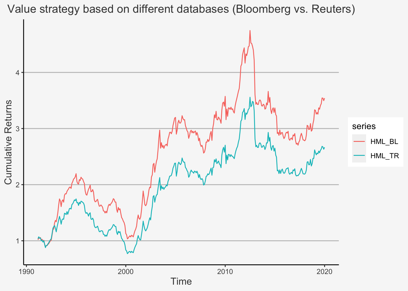
As we can see, although both appear to be correlated and follow the same paths throughout time, we can see that the data provided from Bloomberg (BL) delivers substantially larger factor returns than the data from Thompson Reuters. Let’s look at where these differences arise.
# Let's check why the two HML differentiate that much
CH_data_total_mont_check %>%
  mutate(Total_Eq_t = Total_Eq_t/1000) %>%
  select(Ticker, Date_t, Total_Eq_t, Total_Eq_Real) %>%
  mutate(Diff_Equity = round(Total_Eq_t - Total_Eq_Real,3),
         Diff_Equity_Ratio = round(Diff_Equity / ((Total_Eq_t + Total_Eq_Real)/2),3),
         Same_identifier = ifelse(Total_Eq_t == Total_Eq_Real, 1, 0)) %>%
  subset(Same_identifier == 0) %>%
  # As we can see, there are 16'040 observations where the Total Equity value is different from one another
  subset( abs(Diff_Equity_Ratio) > 0.1) %>%
  # If we now only consider large discrepancies (more than 10% deviation), we obtain 2'255 observations
  subset(abs(Diff_Equity_Ratio) > 0.1) %>%
  # If we only consider the companies which have at at least one point in time a deviation of more than 10%, we would get 51 companies with a deviation of
  # more than 10%!
  select(Ticker) %>%
  unique() %>%
  arrange(Ticker)
## # A tibble: 115 × 1
## Ticker
## <chr>
## 1 ABBN
## 2 ACUN
## 3 ADEN
## 4 ADVN
## 5 ADXN
## 6 AEVS
## 7 AIRE
## 8 AIRN
## 9 ALCN
## 10 ALPH
## # … with 105 more rowsIf we look at the HML factor, we understand that discrepancies can either arise in the Book Value or Market Capitalisation, whereas the Market Capitalisation consists of the Number of Shares as well as the unadjusted Share price. Although we don’t show it here, the Market Capitalisation data is very similar for both data providers, which implies that the discrepancies in returns arise based on the company Book Value. If we drill down on this metric, we can observe that for 16’400 observations the Book Value (Total Equity) is different depending on the database. Let’s now assume that the cumulative return discrepancies are mainly caused by large differences (e.g. >10%) in Book Value. If we consider this, then we understand that 2’255 observations have a discrepancy of more than 10% for the book value, and that, overall, 115 companies show to have a deviation of more than 10% for the book value at least at one observational period. This is striking, as it shows that, even for two of the most mainstream data providers there appears to be large differences in data availability and calculation of basic accounting numbers such as a company’s book value.
Consequently, we can highlight the importance of cross-referencing and double checks with this simple exercise. Therefore, it is advisable to always stick to at least two calculation as well as database options when constructing factors. Based on that, you can then decide which strategy appears more reasonable for the task at hand.